|
|
|
Abstract
This article examines the impact of the regulator’s statement requesting EU insurers to suspend dividend distributions due to the COVID-19 pandemic on share prices of insurance companies. The purpose of the regulation was to maintain a high level of capitalisation of insurance companies, thus allowing them to pay compensation for any damage incurred during the crisis. The statistical significance of the potential negative impact was explored using event study methodology. The empirical results suggest that the negative impact following the statement’s release is not statistically significant over the chosen event window. The robustness of the results is confirmed by several statistical tests – parametric and nonparametric. The measure did not result in a fall in share prices in line with economic theory but, rather, contributed to ensuring the financial stability of the European insurance sector, supporting the real economy and consequently allowing quicker economic recovery.
Keywords: COVID-19; regulator’s statement; insurance companies; event study; share prices
JEL: G28, P43, G22
1 Introduction
The financial stability of the insurance sector is essential in order to ensure access to insurance services. The importance of the insurance sector and of its financial stability is even greater in the current times of uncertainty, during a pandemic. Safeguarding the stability of this sector is relevant from a business continuity perspective and from an individual’s perspective. Nowadays one could not imagine a situation in which an insurance company would not be able to make payment on a health insurance claim. However, in pandemic times such a situation might arise. To minimize the risk of the occurrence of such situations, the European and Occupational Pensions Authority (EIOPA) has urged insurance companies to halt dividends, buybacks and bonuses.
This article examines the impact of this statement, a recommendation requesting EU insurers to temporarily suspend dividend distributions due to the COVID-19 pandemic on share prices of insurance companies. The main event is the release of a statement by EIOPA requesting (re)insurers to temporarily suspend all discretionary dividend distributions and share buy-backs aimed at remunerating shareholders. In its core, the regulation is not extremely binding if compared with the restrictions on dividend payments published by the European Systemic Risk Board in June 2020. The EIOPA statement or instrument, proportionate to the perceived risks (binding instrument, recommendation, opinion), is aimed at limiting dividend distributions for the years 2019 and 2020 of insurance and reinsurance companies doing business in the European Union. The purpose of the regulation was to maintain a high level of capitalisation of insurance companies, thus, allowing them to pay compensation for any damage incurred during the crisis. EIOPA stresses that this macro-prudential measure contributes to increasing the resilience of the financial infrastructure to financial shocks, maintains financial stability and prevents the emergence of disruption in the financial system with the potential of serious negative consequences for the functioning of the financial system and the real economy (OFS,  2020 2020).
As EIOPA stressed, the purpose of the released statement is to maintain a high capital adequacy ratio enabling smooth payment of potential claims during the crisis. However, proactive regulation could also have an opposite effect. The value of equity, i.e., share price, could fall, which might deter potential new investors in the insurance sector and even encourage current investors to sell their shares. To understand the importance of EIOPA’s regulation in its entirety the general circumstances in the insurance sector in the first half of year 2020 should be outlined. Firstly, European insurance companies experienced a slowdown in gross premiums written in 2020, especially in the life sector. Secondly, claims payments increased in the life sector and declined in the non-life sector. Thirdly, the assets of insurers remained mainly invested in bonds. And finally, insurers in the main achieved positive investment gains despite COVID-19 (OECD, 2021).
The aim of the article is to evaluate the issued statement from an economic and a mathematical point of view. Hence, the research question is whether and how the statement requesting insurers to suspend all discretionary dividend distributions and share buy-backs aimed at remunerating shareholders influenced the fall in stock prices of listed insurance companies. A similar challenge was addressed by Petr Jakubik in the article ‟The Impact of EIOPA Statement on Insurers’ Dividends: Evidence from Equity Market” (Jakubik, 2020). Jakubik’s article focuses on the relevant issue regarding the influence of regulations of dividend distributions on the European insurance companies. However, in the present study, I tackled the problem a bit differently. I collected data for 33 European insurance companies from the Bloomberg Terminal. The problem was then explored using event study methodology.
The paper is organised as follows. The next section provides the theoretical framework. The third section describes the data sample, i.e., collection of data and data cleaning, while the event study methodology is presented in the fourth section. The penultimate section includes a presentation of the results with discussion. The last section is the conclusion.
2 Theoretical background: the influence of an imposed ban on the volatility of the financial market
2.1 Economic aspect
In recent years many economic studies have been published examining the influence of a ban or recommendation, issued by governments or international institutions to financial organisations, on the volatility of the financial market (e.g., Baumann and Nier, 2004; Blinder et al., 2008; Shaffer, 1995, and others). These studies analyse indirect disclosure of information about the current financial situation of the economy on various levels, such as company level, national level or even the global level, in the case of the coronavirus crisis. The form of communication of large financial institutions plays an important role when adopting and publishing a regulation since it has the ability to influence the monetary policy and consequently the movement of the financial markets. However, the large variation in communication strategies across financial institutions suggests that a consensus has yet to emerge on what constitutes an optimal communication strategy (Blinder et al., 2008).
Greenspan ( 2003) stresses that banking and insurance companies are at core non-transparent, which cannot be drastically changed by increasing disclosures of information. Moreover, there is no evidence that an increased amount of disclosed information will be sure to increase transparency. It will hold true only on the assumption that the financial market participants correctly interpret the received information, then reasonably put this information in the context given, and finally, respond optimally considering the situation, which is unlikely to occur in practice. Moreover, Baumann and Nier ( 2004) emphasise that stock price volatility can be an appropriate measure of uncertainty among investors and that disclosure of information can reduce stock price fluctuations. Under their assumptions, an increase in the amount of information disclosed decreases the information asymmetry and uncertainty in the financial markets.
Additionally, Schaffer, in one of his studies ( 1995), calls attention to the fact that disclosures of information are often cited as particularly costly. The cost of the disclosure includes direct costs; these occur first, when preparing the disclosure, and second when the disclosure occurs. Regarding the event explored in this article, direct costs are costs incurred during the preparation and at the disclosure of EIOPA’s statement. Likewise, indirect costs are of great importance too (Baumann and Nier, 2004). They occur when companies use given information to participate more profitably in the financial markets. It is for this reason that banking and insurance companies respond to the disclosures with extreme caution.
As mentioned in the previous section, the disclosure that I will explore in this article was already explored by Jakubik ( 2020). He believes that the statement could help to reduce uncertainty about potentially adverse evolutions of solvency positions incapable of absorbing the shocks during the crisis. Furthermore, he obtained empirical results that suggest that the negative impact following the announcement was not statistically significant in the chosen time interval.
2.2 Mathematical aspect
In addition to the economic studies, analysing the influence of an imposed ban or recommendation on the volatility of the financial market, described in the previous section, there are also various mathematical methods. The best known among them is an event study. This is a statistical method used to assess the impact of an event on the value of a company or its stock price (Hayes, 2020). The earliest studies on event study methodology were published in the 1930s and were later on further developed (e.g., Dolley, 1933; Myers and Bakay, 1948; Fama et al., 1969; Brown and Warner, 1985, and others).
The author of the first published event study, Dolley ( 1933), examined stock splits between the years 1921 and 1933. He analysed the influence of stock splits on stock prices. He found out that stock splits, i.e., an increase in the number of stocks, decrease the price of a single stock. He also noted that the total value of all stocks remained almost unchanged during the observed period. As this is the first conducted event study, the statistical basis was not refined, and thus, the results were not satisfactory in terms of reliability and accuracy.
A similar problem was addressed by Myers and Bakay ( 1948). They wanted to find out whether a company’s decision about a stock split influenced its market price. As key impact factors, they indicated the splitting ratio, industrial development at that time and price range following the split. They concluded that in the case of a favourable decision time frame, there might be a positive impact observed, even if a minimal one.
Fama et al. (1 1969) carried out one of the most comprehensive event studies in which they demonstrated that in the past, stock splits were usually related to higher dividends. Their study has proved that stock markets use the announcement of stock split to re-evaluate the expected returns. The authors of the above-mentioned study pointed out that the daily stock return for individual security exhibits substantial deviations from normality, which cannot be noticed when observing monthly data. This suggests that distributions of daily returns are fattailed relative to a normal distribution.
This finding was supported a couple of years later by Brown and Warner ( 1980; 1985), who used a more modern methodology. Moreover, they added that the daily stock returns differentiated substantially from the usual stock returns in the measures of shape – skewness and kurtosis. They upgraded the already existing research with a random selection of event dates and stocks to simulate event study without any assumption about the distributions of stocks returns. Subsequent event studies, mostly conducted in the new millennium, also examined other events, with particular focus on events in companies (such as changes in the management, the amendments to the Statute, mergers and acquisitions, and others).
3 Data sample
Secondary data, dividend payments and share prices, are obtained from the Bloomberg Terminal database (2020). Firstly, I explored the dividend policy before this event, which was relatively stable, since in the last few years there was no economic crisis. The last significant one was the financial crisis of 2007-2008. However, there were some individual market shocks, such as the rise of cryptocurrencies, oil crashes and jumps, reopening of the Greek stock market and others (The Center for Financial Stability, 2021).
Secondly, I checked what the actual decision was after the statement was issued – whether insurance companies really suspended dividend distributions. The percentage of companies that paid out dividends regardless of the recommendation is 49%. As an example, payments and non-payments of dividends for insurance company Sava Re are presented in figure 1.
Figure 1Payment of dividends – Sava Re DISPLAY Figure
Thirdly, I cleaned the data of share prices, all non-trading days (Saturdays, Sundays and major holidays) and the insurance companies with missing data were removed. Then, I calculated the return on the share, expressed as a percentage, for each day. From here on, the R programming language and the RStudio development environment were used, partially edited data and S&P index values were imported into R. Next, I cleaned the data using standard methods and compiled an organised database on which I performed an event study.
4 Event study methodology
In this article, I decided to use the event study methodology for assessing the impact of an event on the value of stock prices. As already mentioned in section 2, event study methodology is a statistical method for analysing the influence of a particular event on a company’s value or its stock price (Hayes, 2020). Following Henderson (1990), event studies are typically arranged into four groups: - market efficiency studies – these are based on the analysis of the speed and the correctness of the response,
- information value studies – these want to find out to what extent the event is reflected in the stock price,
- metric exploration studies – these studies split data into subsamples and look for abnormal returns in the subsamples,
- methodological studies – these strive to find the most efficient method for taking into consideration the specificity of the data.
The event study conducted in this article falls under information value studies. The aim is to determine to what extent the event of the release of a statement issued by EIOPA requesting insurers to suspend all discretionary dividend distributions is reflected in the stock prices of insurance companies. According to Damodaran ( 2012), events can be general (impact on the whole market) or specific (impact on a particular company). The event explored in this article, is at core, a general one. However, given the limitation of scope, the event will be addressed more specifically. Sample size determination is based on the principle that the accuracy of estimates increases rapidly when the sample size increases. For that reason, the sample contains all 33 European insurance companies data for which are available in the Bloomberg Terminal. The event study design, according to Damodaran ( 2012), involves the following steps: 1) event definition 2) examination period definition 3) calculation of abnormal returns 4) data smoothing 5) aggregation of abnormal returns 6) testing procedure.
I followed the scheme above while conducting my event study.
4.1 Event definition
In the first step of the research process, the event, which will be explored further below, must be clearly defined. In the examined case, the published information is in the form of a statement issued by EIOPA requesting insurers to suspend all discretionary dividend distributions. The statement was published on April 2nd 2020.
On the one hand, supervisory institutions of some European member states (MS) responded even earlier on their own initiative. On the other hand, other MS to which the coronavirus spread later responded to the issued statement with a delay. For individual European MS, I looked up the internal dates of the publication of the regulation and arranged the data systematically (table 1) so that the dates coincide on the so-called day 0 (the day when the regulation was issued).
The dates of the issued regulations range from the 24th of March to the 7th of April 2020 (table 1). The first regulations were issued by Germany and Finland, the last from the chosen European MS to respond was Belgium. A one-month gap between the first and the last response would be expected since the epidemiological situation varied among European MS (Steward, 2020).
Furthermore, the responses were similar, but still different across member states; some responses seem to be less strict than the EIOPA statement with respect to dividend distribution, for example Germany, Ireland, Italy, Norway and the United Kingdom (ESRB, 2020). The reason for the differences in strictness could be that these European MS are the home states of some of the biggest and the most successful insurance companies in Europe. Therefore, their national regulators probably trusted in their decisions and were not afraid that the possible payment of dividends would result in a low capital adequacy ratio.
Table 1Dates of the issued regulations of the chosen European member states DISPLAY Table
4.2 Examination period definition
The second step is based on the definition of the examination period around the studied event. In a case in which there is less information about the event date, the examination period is wider. Since the date for the studied event is known, I decided to gather daily data. The method is more accurate if the length of the examination period is approximately 250 days (Brown and Warner, 1985). That being the case, I have chosen the following beginning and end of the period under examination: the 24th of June, 2019 and the 12th of April, 2020. Considering the above-mentioned systematic data compilation (the coincidence of day 0) and the exclusion of the nontrading days, the length of the time period is 250 days. In addition, the starting date is about four months before the first case of coronavirus infection was identified in the World, thus, when the European financial markets were relatively stable. In mid-May 2020, which marks the end of the time period, the majority of European MS had already coped with the first wave of the coronavirus pandemic. The period under examination is presented graphically in figure 2. Other significant events, which accompanied the beginning of the coronavirus crisis, are added as well.Figure 2Examination period DISPLAY Figure
It is worth remembering here that day 0, in the case of the majority of European MS, came after the 2nd of April 2020 when EIOPA issued the statement, although there are some European MS that responded earlier, meaning before the 2nd of April 2020. In the case of these MS, the last and the penultimate points on the timeline should be replaced.
The chosen examination period is usually divided into two parts: the estimation period and the observation period. The estimation period is in general defined as the time from day t0 to day t1, while the observation period is defined from day t2 to t4 (Brown and Warner, 1985). Day 0 is marked with t3 on the timeline (figure 3).
Figure 3Examination period in general DISPLAY Figure
In our case, the estimation period is defined as the time from day -244 to day -6, while the observation period is defined from day -5 to day +5. The timeline is presented in figure 4.
Figure 4Examination period in general DISPLAY Figure
To check the adequacy of the endpoints of the observation period, I plotted the graphs of market returns for the chosen 33 insurance companies. As an example, there are two graphs plotted in figures 5 and 6 for two insurance companies: Generali (Italy) and Hiscox (United Kingdom). The estimation period is marked grey; black is used for the observation period. In both graphs, there is a dynamic change of movement around day -25. The reason behind this jump is the coronavirus outbreak in Europe. It is important that the event of the coronavirus outbreak is separated from the event of the issued statement, so the results will be more robust.
Figure 5Stock returns Generali DISPLAY Figure
4.3 Calculation of abnormal returns
The third step of the event study assesses the abnormal returns on a stock (occurring as a result of the event). To assess these, the so-called ‟normal” or actual returns on a stock have to be defined first. An actual return on a stock Ri,t of the insurance company i on the day t refers to the actual gain or loss an investor in the insurance company i experiences on the day t. Furthermore, the abnormal return on a stock ARi,t of the insurance company i on the day t is defined as the difference between the actual return (Ri,t) and the expected return (E(Ri,t|Xt), where Xt stands for the vector of explanatory variables (e.g. market index) in day t), t ∈ [-5,5], | ARi,t = Ri,t - E(Ri,t│Xt). | (1) |
4.3.1 The mean adjusted returns model
The basic assumption of the mean adjusted returns model is that the vector of explanatory variables Xt is constant (independent of time t). The expected return (E(Ri,t|Xt)) on the stock of insurance company i can be written as average actual return on the stock of insurance company i: 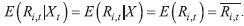 | (2) |
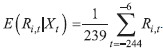 | (3) |
4.3.2 The market adjusted returns model
The market adjusted returns model is based on a chosen stock market index, I have chosen the usual index S&P 500 (Standard & Poor’s 500 Index), which is used quite often when conducting event study. The expected return, (E(Ri,t|Xt)) on the stock of insurance company i on the day t, in the market adjusted returns model is defined as market return (RM,t), i.e., the value of the chosen index on day t: | E(Ri,t│Xt) = RM,t = S&Pt | (4) |
4.3.3 The risk adjusted returns model
The last chosen model for calculating the expected returns is the risk adjusted returns model, which is based on the following linear regression model| Ri,t = αi + βiRM,t + ei,t | (5) |
 | (6) |
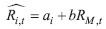
The regression analysis, computed on the data of 33 chosen insurance companies, indicated that the estimator of the regression constant (ai) is statistically insignificant. Thus, I decided to remove this term from the regression equation. After a detailed analysis, I found out that the explanatory power of the regression model is even higher when the estimator of the regression constant is eliminated. The elimination is reasonable also because it is likely that when the market return equals zero, the actual return equals zero as well. This is graphically confirmed by regression scatterplots. Figures 7 and 8 illustrate data on two examples.
Figure 7Regression scatterplot – Direct Line (UK) DISPLAY Figure Figure 8Regression scatterplot – Allianz (Germany) DISPLAY Figure
The new regression models, where the explanatory variable is market return, explain between 40 and 70% of the variability of the actual return, which is within the estimated interval for regressions performed on financial data (Fernando, 2020).
Thus, the expected return, ( E(Ri,t| Xt)) on the stock of insurance company i on the day t, in the risk adjusted returns model, is defined as follows | E(Ri,t│Xt) = ai + biRM,t = ai + biS&Pt | (7) |
4.4 Data smoothing
Data smoothing removes noise and other microstructures from a data set and allows important patterns to stand out. When a time series is smoothed, the dynamics of the observed phenomenon are clearer. In this study, the time series of abnormal returns y1, y2, …, yT (in the observation period) were smoothed with moving averages of order k by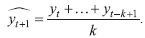 | (8) |
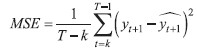 | (9) |
4.5 Aggregation of abnormal returns
The fourth step of an event study focuses on the impact of the event at an aggregate level. The aggregation of the abnormal returns is done over securities (index i). The average abnormal return of n insurance companies on day t (AARt) is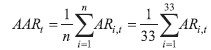 | (10) |
 | (11) |
4.6 Statistical tests
To test a hypothesis or assumption about the value of unknown parameters of a statistical variable, two groups of tests can be used – parametric and nonparametric (Neideen and Brasel, 2007). The most favourable situation is that the components of the sample are independent and (approximately) normally distributed (Serra, 2004). In this study the values of the basic sample represent actual returns on stocks (Ri,t). On this basis I then calculated abnormal returns (ARi,t) which represent upgraded sample. The fulfilment of the assumption of independence is extremely difficult to justify in practice, so here I will assume it for simplicity. However, I have explored the normality assumption in more detail.
The estimation period in the event study also covers an important event of the coronavirus outbreak in Europe, which shook the financial markets (section 4.2). Due to the large impact of the outbreak on the stability of the estimation period, I excluded this event from the stable period (but not from the estimation period) since the parametric tests are based on the estimation period. Thus, the stable period is the time interval [-250, -50].
The histogram of average abnormal returns in the stable period indicates a deviation from the normal distribution. This is also confirmed by the measures of shape – skewness and kurtosis. The skewness value is 0.4301, and the value of kurtosis equals 1.0791. None of the three tests: the Jarque-Bera test, the D’Agostino-Pearson test and the Anderson-Darling test, rejected the hypothesis of the normal distribution. However, due to the financial nature of the data, I suspected that there might be a possibility of heavy tails (Brown and Warner, 1985), which occur commonly in finance.
A heavy-tailed distribution is a distribution whose tail falls toward zero slower than the exponential function. In general, heavy tails show a deviation from the normal distribution cause by extreme events. The heavy tail is indicated on the intervals (-3, -1) and (1, 3) on the primary axis of the theoretical quantiles.
I approached the problem of heavy tails with non-linear data transformation with a generalised iterative method of moments (IGMM). This transformation results in the skewness value closer to zero and the kurtosis value closer to three (LambertW, 2020). After, I checked the normality again with standard normality tests and by plotting ‟Q-Q Plot” (figure 9).
Figure 9Q-Q Plot of the transformed average abnormal returns in the stable period DISPLAY Figure
The heavy tail on the interval (-3, -1) has almost disappeared, and a minor change is also noticed on the interval (1, 3). To perform the above-mentioned transformation, I have used the LambertW software package in R. The parametric two-sided t-test was then performed on the transformed data. The t-test tests the null hypothesis H0 versus the alternative hypothesis H1: where the value μ0 is taken from the stable period. Thus, the null hypothesis is that the mean of the average abnormal returns in the observation period equals the mean of the average abnormal returns in the stable period. Moreover, the null hypothesis that the median of the average abnormal returns in the observation period equals the median of the average abnormal returns in the stable period is tested by the nonparametric sign test. This means that the number of negative average abnormal returns is equal to the number of the positive average abnormal returns: | | H0: Me = Me0 | and
| H1: Me ≠ Me0, |
where the value Me0 is the median of the sample of average abnormal returns from a stable period.
The values from the stable period are real and are not transformed, as in the case of the t-test. The key difference between the sign test and the t-test is that the results of the sign test will also reveal information about the statistical significance of the negative or positive average abnormal returns since the sign test takes into account the sign of the difference of the observations from the median.
Since the sign test takes into account only the sign of the differences of the observations from the median, I also performed the Wilcoxon signed-rank test, which considers the size of the differences of the observations from the median. The hypothesis tested is that the number of negative average abnormal returns is equal to the number of positive average abnormal returns:
| | H0: Me = Me0 | and
| H1: Me ≠ Me0, |
where the value Me0 is the median of the sample of average abnormal returns from a stable period.
Additionally, I conducted a parametric t-test to test the hypothesis that the mean of the CAAR in the observation period is equal to the mean of the CAAR in the stable period | | H0: E(CAAR) = E(CAAR0) | and
| H1: E(CAAR) ≠ (CAAR0). |
5 Results and discussion
I conducted an event study on a sample of 33 European insurance companies. The abnormal returns of individual insurance companies in the observation period are presented in table 2. On average, the number of days in the observation period when negative abnormal returns were observed in 5 days, which is less than half of the days in the observation period. The most negative abnormal returns (in 10 out of 11 days) were indicated in case of Hiscox (UK). By contrast, Vienna I. G. (Austria) and KBC I. G. (Belgium) had zero days when the abnormal returns were negative. Since Vienna Insurance Group and KBC Insurance Group are some of the largest insurance companies in Europe, suspending discretionary dividend distributions in order to absorb the shocks for this insurance company was not necessary. The companies and their shareholders were confident of enabling smooth payment of the claims during the crisis. In case of Vienna Insurance Group this was later confirmed, as they paid out all dividends.
Moreover, I have compared the behaviour of the stocks in the sample that pay significant dividends to those that pay little or nothing. The analysis shows that higher values of abnormal returns were observed in case of insurance companies that pay significant dividends (dividend yield is more than 4%). As expected, lower abnormal returns were observed in other insurance companies with a dividend yield under 4%. It is intuitively clear that shareholders expecting higher dividends would be more concerned about the issued statement, than those expecting lower dividends.
Furthermore, it is important to stress that the most significant divergences of 0 abnormal returns were positive abnormal returns. The highest positive abnormal returns exceeded the limit of 7%, mostly on days -5 and -4. The majority of the insurance companies with such results were from the UK. Many UK investors poured billions of dollars into insurance companies at that time because they thought that the pandemic would ultimately prove the catalyst that ends a period of low returns for the industry. Their belief was that the claims incurred during the pandemic would not overwhelm insurance companies. Yet, those claims might allow insurance companies to justify price rises for new policies (Ralph, 2020). It is important to bear in mind that the abnormal returns calculated might not be statistically significant, which means they could be random. Thus, the performance of the following statistical tests is crucial.
The values of t-test statistics are the lowest on days -2 and -1 (table 3). The reason for this might be that the majority of European MS responded to the statement issued with delays (section 4.1). For the majority of MS, EIOPA issued the statement a few days before day 0, and with a delay of a couple of days, the national regulators responded. The results are not statistically significant. Therefore, the hypothesis that the expected value of average abnormal returns in the observation period is equal to the expected value of the average abnormal returns in the stable period can be rejected. Hence, we cannot reject the null hypothesis that the issued statement doesn’t affect stock prices of insurance companies at the 0.05 significance level.
Table 2Abnormal returns for the chosen 33 European insurance companies (in percentage) DISPLAY Table Table 3T-test DISPLAY Table
As data from the stable period was transformed (section 4.6), two more nonparametric tests were performed to justify the robustness of the t-test results. Again, the values of nonparametric sign-test statistics are the lowest on days -2 and -1 (table 4). The null hypothesis that the median of the average abnormal returns in the estimation period is equal to the median of the average abnormal returns in the stable period cannot be rejected at the 0.05 significance level. Therefore, we cannot argue that the number of negative average abnormal returns doesn’t differ from the number of positive average abnormal returns.
Table 4Sign test DISPLAY Table
To complement the sign test, I performed a nonparametric Wilcoxon test (table 5). The results are not statistically significant. Thus, we cannot reject the null hypothesis that the median of the average abnormal returns in the observation period is equal to the median of the average abnormal returns in the stable period at the significance level of 0.05. Furthermore, we cannot reject the proposition that the number of negative average abnormal returns equals the number of positive average abnormal returns.
Table 5Wilcoxon signed-rank test DISPLAY Table
The alignment between the statistical significance of the results is noticed, since there is no statistical significance at all. The results of the t-test suggest that the issued statement did not have an impact on the share price of insurance companies. Moreover, according to the sign test, we cannot claim that the number of negative average abnormal returns is different from the number of positive average abnormal returns. Lastly, the Wilcoxon signed-rank test confirms both – the sign and the t-test.
As mentioned in the previous section, a parametric t-test was conducted to study the reactions of the insurance companies selected. I have tested whether the expected CAAR of each insurance company was equal to or different from the expected CAAR of this company in the stable period. In almost 60% (19 cases among 33) the hypothesis cannot be rejected. However, it is important to mention three European MS: Finland, Belgium and The Netherlands, all with the p-values below 0.05. Insurance companies from these MS have the highest dividend yields (above 4%) and the greatest absolute values of CAAR resulting in statistical significance and the possibility of rejecting the hypothesis for those companies. Yet, as stated, the hypothesis cannot be rejected in the majority of cases. Thus, the expected CAAR of each insurance company is equal to the expected CAAR of this company in the stable period at the significance level of 0.05.
Table 6T-test for CAAR DISPLAY Table
Since Jakubik, in his article presenting the source literature, performed different statistical tests than the ones presented in this study, it is very difficult to compare the results. However, Jakubik’s conclusions align with mine. The null hypothesis that the issued statement does not affect stock prices of insurance companies could not be rejected either by my results (the observation period is 11 days long) or by Jakubik’s results (the observation period is 13 days long).
Similar conclusions have been drawn in the banking sector. Giese, Haldane and Jakubik ( 2020) stress the crucial importance of financial resilience for the economy, for example, in the form of buffers of capital and liquidity. Without a strong and flexible prudential regulatory regime, financial resilience would be outstandingly lower. Similarly, their study confirms that regulations did not have a significant negative impact on the share prices. Likewise, in the year 2020, no European insurance company following EIOPA’s recommendations encountered liquidity problems, suggesting strongly that the issued statement fulfilled its purpose without undesired side-effects.
This research, however, is subject to several limitations, especially methodological. First, the issue of sample bias must be addressed. As I had limited access to data, my sample (consisting of 33 European insurance companies) does not fully reflect the general population of European insurance companies. The sample would be more random and the results more robust if the sample size was larger. Second, prior research that is relevant to my article is quite limited as there is little research analysing the regulator’s statements in the insurance sector on stock prices. However, prior studies have analysed the impacts of EIOPA recommendations on pension plans and products in the conditions after the economic crisis (Bejaković, 2020). I believe that my finding is still reliable and valid despite these limitations. A possible way to overcome some of these limitations in future studies is the use of various methods, not only the event study. One of the possibilities could be the analysis of covariance (Hogan, 1996) or latent variable model (Acharya, 1993).
6 Conclusion
In recent decades, the need to analyse financial market response to disclosures of important information has been growing. For financial market participants (investors), such analyses are useful because they enable more accurate forecasting of market movements and consequently the choice of less risky or more profitable investments. The financial market response to disclosure has already been the subject of much research. However, there is relatively little research conducted on the effects of regulatory statements. Most studies conducted in the field focus on the banking sector; the number of those analysing the insurance sector is almost negligible. The article, therefore, represents an important contribution to this evolving field of financial governance.
The findings of this article are useful for regulators and investors as they demonstrate the effects of regulatory statements on financial stability. Hence, the article shows that insurance regulators should in future put their trust in the economic theory that market investors make a rational assessment focusing on long-term rather than short-term profit. Therefore, regulators in the European insurance sector can take drastic measures in order to ensure financial stability without any fear of a severe fall of stock prices. Which is of course not the case in all economic sectors. Furthermore, from the investors’ perspective, an investment in the European insurance sector is a great addition to any investor’s stock portfolio. As presented in this article, the insurance business has the potential to produce excellent long-term returns, since this business works well in strong economies, during recessions, etc. This is so because of a specificity of the insurance sector as such and because of a strong and engaged regulator protecting the financial markets even during the pandemic.
The COVID-19 pandemic negatively affected the solvency of insurance companies and consequently increased the vulnerability of the economy. The pandemic is essentially predominantly a public health crisis, which rapidly spiralled into a full-blown economic crisis. However, it is important that it does not develop into a financial one too. As EIOPA stressed, the purpose of the released statement was to maintain a high capital adequacy ratio. This would enable smooth payment of potential claims during the crisis. However, proactive regulation could also have a negative impact on the value of equity, i.e., share price, which would deter potential new investors in the insurance sector. One should bear it in mind that EIOPA’s release of a regulatory statement affected not only the insurance sector but also the economy as a whole. The statement requesting insurers to suspend all discretionary dividend distributions interrupted the cash flow in the economy.
In this article, I examined the impact of the released regulator’s statement on the share prices using the event study methodology on a sample of 33 European insurance companies. Empirical results showed that the negative effects observed immediately after the release of the statement are not statistically significant. The robustness of the results is confirmed by several statistical tests – parametric and nonparametric. I can therefore provide an answer for the research question stated at the beginning of the article and conclude that the statement requesting insurers to suspend all discretionary dividend distributions and share buy-backs aimed at remunerating shareholders did not precipitate a fall in stock prices of listed insurance companies. The finding is consistent with the economic theory that investors make decisions relatively rationally and maximise long-term profit. The issued regulation thus contributes to ensuring the financial stability of the European insurance sector, offers support to the real economy and indirectly enables a faster economic recovery.
Notes
* I would like to express my sincere gratitude to my supervisor, Professor Jaka Smrekar, for his continuous support, invaluable advice and encouragement during my research. The present article is based on a topic, that I discuss mostly from a mathematical point of view in my thesis. I would also like to thank two anonymous referees whose comments have contributed to the final version of the paper.
* I would like to express my sincere gratitude to my supervisor, Professor Jaka Smrekar, for his continuous support, invaluable advice and encouragement during my research. The present article is based on a topic, that I discuss mostly from a mathematical point of view in my thesis. I would also like to thank two anonymous referees whose comments have contributed to the final version of the paper.
Disclosure statement
The author declares that there is no conflict of interest.
References
Acharya, S., 1993. Value of latent information: alternative event study methods. The Journal of Finance, 48(1), pp. 367-382 [ CrossRef]
Baumann, U. and Nier, E., 2004. Disclosure, volatility, and transparency: an empirical investigation into the value of bank disclosure. Economic Policy Review, 10(2), pp. 31-32.
Bejaković, P., 2020. The Future of Pension Plans in the EU Internal Market-Coping with Trade-Offs Between Social Rights and Capital Markets. Public Sector Economics, 44(4), pp. 567-571 [ CrossRef]
Blinder, A. S. [et al.], 2008. Central bank communication and monetary policy: A survey of theory and evidence. Journal of Economic Literature, 46(4), pp. 910-911 [ CrossRef]
Brown, S. J. and Warner, J. B., 1980. Measuring security price performance. Journal of Financial Economics, 8(3), pp. 205-258 [ CrossRef]
Brown, S. J. and Warner, J. B., 1985. Using daily stock returns: The case of event studies. Journal of Financial Economics, 14(1), pp. 3-31 [ CrossRef]
Craig MacKinlay, A., 1997. Event Studies in Economics and Finance. Journal of Economic Literature, 35(1), pp. 13-39.
Damodaran, A., 2012. Investment valuation: Tools and techniques for determining the value of any asset. New York: John Wiley & Sons.
Dolley, J. C., 1933. Open market buying as a stimulant for the bond market. Journal of Political Economy, 41(4), pp. 513-529 [ CrossRef]
EIOPA, 2020. Monitoring of dividends distribution following EIOPA and NCA statements. EIOPA-BoS-20-443, pp. 4-10.
Fama, E. F. [et al.], 1969. The adjustment of stock prices to new information. International Economic Review, 10(1), pp. 1-21 [ CrossRef]
Giese, J., Haldane, A. and Jakubik, P., 2020. COVID-19 and the financial system: a tale of two crises. Oxford Review of Economic Policy, 36, pp. 200-214 [ CrossRef]
Greenspan, A., 2003. Corporate governance. Remarks by Chairman Alan Greenspan at the 2003 Conference on Bank Structure and Competition, Chicago, Illinois, May 8, 2003.
Henderson Jr, G. V., 1990. Problems and solutions in conducting event studies. Journal of Risk and Insurance, 57(2), pp. 282-306 [ CrossRef]
Hogan, S., 1996. Covariance analysis as an alternative event-study methodology. Managerial Finance, 22(3), pp. 54-55 [ CrossRef]
Jakubik, P., 2020. The impact of EIOPA statement on insurers dividends: evidence from equity market. Financial Stability Report, EIOPA 18, pp. 104-120.
Myers, J. H. and Bakay, A. J., 1948. Influence of stock split-ups on market price. Harvard Business Review, 26(2), pp. 251-255.
Neideen, T. and Brasel, K., 2007. Understanding Statistical Tests. Journal of Surgical Education, 64(2), pp. 93-96 [ CrossRef]
Serra, A. P., 2004. Event study tests: a brief survey. Org-Revista Electrónica de Gestão Organizacional, 2(3) pp. 248-255.
Shaffer, S., 1995. Rethinking disclosure requirements. Business Review, 5, 15-29.
|


