|
|
|
Abstract
The relationship between public expenditure and economic growth is one of the central topics in economics literature, and an extensive body of knowledge has accumulated around it. The current consensus is that infrastructure, education and health are the types of public services that are likely to contribute to economic growth. Still, the question of how public resources should be allocated among them remains unanswered. This paper, benefiting from an endogenous growth model that is useful in the identification of the optimal allocation of public resources, analyses the growth effect of the composition of public investment in Turkey using a dataset for the years between 1975 and 2001. Results indicate that, between these years, the government overinvested in transportation and communication services and underinvested in energy infrastructure, education, health, and city infrastructure and security services. There is further evidence that public policy led to an underinvestment in energy infrastructure in these years. The scope of the analysis is confined by the limitations of the economic model. Additionally, the robustness of the results depends on the assumption that public policy is exogenous in the model.
Keywords: public investment; health; education; infrastructure; economic growth; optimal allocation; Turkey
JEL: O52, O40, O20, H50
1 Introduction
Investigation of the relationship between public expenditure and economic growth is a research topic that stems from the origins of the economics discipline itself. Adam Smith’s invisible hand is invoked to oppose government intervention in the economy. Since Smith’s time, the role of public policy in economic growth has been analysed from various perspectives that include the Keynesian and Latin American Structuralist schools, which heavily influenced state-led economic policies in the 1950s and 1960s. However, the debt and financial crises of the 1970s and 1980s led to the Washington Consensus in 1989, which limited the role of government to the provision of infrastructure, education and health. The shift in economic policy was accompanied by empirical studies that linked public infrastructure expenditure to growth, and by the introduction of the endogenous growth theory, which provided arguments in favour of government intervention in the education sector. These developments in economics literature generated the most current consensus: that public expenditure on education, health and infrastructure is likely to contribute to growth as it helps in the creation of human capital and complements private sector investment.
The second point of discussion regarding the link between public expenditure and economic growth is about the composition of public expenditure. How should the resources be allocated among education, health and infrastructure? This aspect of the topic became a focus of attention relatively recently and remains underresearched.
One of the earliest studies on the composition of public expenditure and economic growth was carried out by Devarajan, Swaroop and Zou (  1996 1996), who provide a model of endogenous growth theory that helps to determine whether the government underspends or overspends in a particular type of public service. Although many other scholars (Lee, 1992; Turnovsky and Fisher, 1995; Agénor and Moreno-Dodson, 2006; Chen, 2006; Agénor, 2009; Agénor and Neanidis, 2011) proposed models to analyse the relationship between the allocation of public expenditure and economic growth, the model in Devarajan, Swaroop and Zou ( 1996)has the advantage of having a general framework. It is also the one that imposes the fewest restrictions in the analysis regarding the relationship between the composition of public expenditure and economic growth.
This paper contributes to the literature by applying the model in Devarajan, Swaroop and Zou (( 1996) to a panel dataset of Turkish provinces for the years between 1975 and 2001. It complements the aforementioned study by proposing a regression model to test the theory in question. Additionally, this study differs from Devarajan, Swaroop and Zou ( 1996)in terms of public spending data; while they carry out their analyses using public current and capital expenditure, this study applies this method to the latter.
Turkey is chosen as the subject of the research because of its characteristics. Turkish provinces vary significantly in terms of economic performance. The provinces in the west are considerably more developed than those in the east. To foster the economy in underdeveloped areas, Turkish governments have aimed to increase the accessibility of infrastructure facilities and improve human capital. This policy has been pursued by implementing public investment projects in infrastructure, health and education facilities using the central government budget. Thus, Turkish provinces constitute a sample suitable for use in the analysis of the relationship between the composition of public expenditure and economic growth. As the public policy in question uses public investment projects to promote development, the analysis in this paper concentrates on the link between the composition of public investment and economic growth 1.
The time range of the dataset is narrowed to 1975 and 2001 as the economic growth rates for the provinces are available only for these years. To address reverse causality between public investment variables and the economic growth, the dependent variable is specified as the five-year forward-moving geometric average of the per-worker real GDP growth rate 2. This is also to capture the lagged impact of public investment on the output growth rate. For empirical analysis, the random-effects and the pooled OLS techniques are used. The standard errors are corrected for heteroscedasticity, and serial correlation within and between panels. Post-estimation diagnostics provide evidence for the robustness of the results 3.
The results in this paper show that, for the years between 1975 and 2001, there was an overinvestment in transportation and communication. The policy implication of this study is that, for the investigated time period, Turkish public policy should have shifted resources from this public layout to the provision of energy infrastructure, education, health, and city infrastructure and security services. Results provide additional evidence that the governments between the years 1975 and 2001 underinvested in energy infrastructure.
2 Literature review
Literature regarding the relationship between government expenditure and economic growth focuses on particular types of spending, namely, infrastructure, education and health. The origin of the link between public expenditure on infrastructure and economic growth is an empirical study carried out by Aschauer (1989), who demonstrated that public expenditure on roads and highways has considerable growth effects. This initiated discussions about whether it is the government consumption expenditure that might have growth-reducing effects, and that public policy should favour capital spending, which is understood to be expenditure on infrastructure.
The relationship between public expenditure on human capital and economic growth builds on the endogenous growth theory, which identifies the source of economic growth as technological progress, which is a function of human capital. Endogenous growth models are derived on the assumption that social returns to public expenditure on human capital are higher than private returns to it, and so the equilibrium growth rate in a free-market economy is sub-optimal (Barro and Sala-I-Martin, 1992).
The combination of the two streams of the literature provided above led to the current consensus that public expenditure on education, health and infrastructure is likely to have a positive impact on economic growth. The arguments in favour of government intervention in these sectors can be listed as: market failure in the provision of services in these areas, their high positive externalities, their impact on human capital and thus on research and technology, their positive impact on private sector productivity, and their welfare benefits. However, it is also acknowledged that public investment might crowd-out private investment. Additionally, public investment is considered less efficient than private investment due to factors such as rent-seeking, corruption and congestion.
The literature that analyses the relationship between the composition of government expenditure and economic growth is divided in accordance with the streams of the literature that focus on the link between public expenditure and economic development. While some investigate the composition of public expenditure by disaggregating it as capital and consumption spending (Lee, 1992; Turnovsky and Fisher, 1995), others focus on the functional composition of public expenditure as health, education and infrastructure (Agénor and Moreno-Dodson, 2006; Chen, 2006; Agénor and Neanidis, 2011; Agénor, 2009 ).
Correspondingly, in the relevant empirical literature, the majority of studies focus on the relationship between public capital expenditure and economic growth (Haque, 2004; Gupta et al., 2005; Ghosh and Gregoriou, 2008; Afonso and Furceri, 2010; Chamorro-Narvaez, 2012). Few studies further investigate the growth effect of public expenditure on infrastructure services such as transportation facilities (Shioji, 2001; León-González and Montolio, 2004; Pereira and Andraz, 2005). There are relatively few studies that include public health and education spending in empirical analysis (Easterly and Rebelo, 1993; Odedokun, 2001; Ramirez and Nazmi, 2003; Bose, Haque and Osborn, 2007). Although the results regarding the impact of public capital on economic growth are mixed, overall findings in the literature appear to support the hypothesis that public expenditure on transportation is positively related to growth. The literature also provides evidence that public education expenditure is positively associated with economic progress.
In this literature, Devarajan, Swaroop and Zou ( 1996) provide a model that encompasses all others as it can be used to analyse the composition of any type of public expenditure. The authors relate the productivity of a type of public expenditure to its share in total public expenditure, and the productivity of other types of public expenditure in the model. Despite the strength of their model, the results in Devarajan, Swaroop and Zou ( 1996)are unconventional and their robustness is debatable. The authors find a positive relationship between public consumption expenditure and economic growth, which contradicts the implications of economic theory. Their results also indicate a negative growth effect for public expenditure on education. Haque ( 2004) observes that Devarajan, Swaroop and Zou ( 1996) do not account for unit roots in the data, which may have biased their results.
This paper contributes to the literature by applying the model provided by Devarajan, Swaroop and Zou ( 1996) to public investment (i.e. public capital expenditure) for a panel dataset of Turkish provinces for the years between 1975 and 2001. This study also proposes a regression model to test the theory in question to obtain robust results. The shortcomings of the regression model used in Devarajan, Swaroop and Zou ( 1996) are discussed in more detail in the relevant section.
3 Economic model
The economic theory adopted in this paper is provided by Devarajan, Swaroop and Zou (1996). For the purposes of this paper, this section presents a brief summary of that model, together with a conclusion that relates the composition of public expenditure to economic growth.
Devarajan, Swaroop and Zou ( 1996) use an endogenous growth model, in which the household intertemporal utility function, U, equals:
where ρ is rate of time preference, ρ > 0, and the utility function is:
In the utility function, σ is the elasticity of intertemporal substitution, and is assumed to be constant.
The authors use a production function that has the constant elasticity of substitution property:
| y = [ak–r + bg1–r + δg2–r]–1/r |
|
where y is total output per capita, and g1 and g2 are the components of public expenditure per capita, respectively. The terms a, b and δ are productivity parameters, while r is a function of elasticity of substitution, 
In the model, the income tax rate ( τ) and hence the share of total public expenditure in output  are considered given. The government’s budget constraint is defined as:
where
| g1 = θτy, (0 ≤ θ ≤ 1), and so g2 = (1 – θ) τy |
|
The constraint for capital accumulation is specified as:
which shows the amount of income per capita after taxation and consumption.
Devarajan, Swaroop and Zou ( 1996) find the condition for an increase in the share of g1 in total public expenditure to have a positive impact on economic growth as in:
which simplifies to:
if the value of r equals 0 (i.e. the elasticity of substitution equals 1), in which case, the production function corresponds to the Cobb-Douglas production function.
The inequality indicates that an increase in the share of g1 in total public expenditure, θ, will result in higher growth only if the ratio of the output elasticity of g1 to g2,  is higher than the ratio of θ, the share of g1 in total public expenditure, to (1 – θ), the share of g2 in total public expenditure, 
This suggests that, even though the output elasticity of g1 was higher than the output elasticity of g2 – that is, a 1% percent increase in g1 created a higher increase in output than a 1% increase in g2 did – if an increase in the share of g1 in total public expenditure results in the violation of the inequality condition above, then an increase in the share of g1 in total public expenditure will not have a positive effect on economic growth.
It can be seen that the model does not depend on any initial assumption regarding the productivity of g1 and g2. Any component of public expenditure can be productive if its share relative to other components satisfies the condition above. Productivity of public expenditure is not a matter of the sector in which it would be expected to have a positive impact on growth. Thus, the productivity of public expenditure in this model is in relative terms, which implies that public expenditure in some sectors that would be considered to contribute to growth may turn out to be detrimental to it if the composition of public expenditure is taken into account.
As this paper uses public investment data, in its context of analysis, g1 and g2 correspond to the components of public investment. Then, Devarajan, Swaroop and Zou’s ( 1996) model shows that, for a given budget, if increasing the share of g1 in g is negatively associated with economic growth, then there is an overinvestment in the first type of public investment. Similarly, for a given budget, if increasing the share of g1 in g is positively associated with economic growth, then there must be an underinvestment in the first type of public investment. Thus, the model provides a tool for assessing Turkish public policy regarding the implementation of public investment projects in different sectors and balancing the shares of public investment accordingly for the years between 1975 and 2001.
4 Regression model
This section discusses possible regression models that can be used to apply the theoretical model to data. The theoretical model in Devarajan, Swaroop and Zou (1996) assumes that there are two types of public expenditure. Type 1 is denoted by g1, and type 2, by g2. The model shows the conditions for a change in the share of a type of public expenditure, for a given share of public expenditure in GDP (g/y), to have a positive impact on economic growth, γ. Thus, the growth effect of a type of public expenditure depends on: (1) its share in total public expenditure, (2) its productivity, and (3) the productivity of the other type of public expenditure.
Devarajan, Swaroop and Zou ( 1996) assume a linear regression model for empirical
analysis, and include the shares of each component in total public expenditure and the share of total public expenditure in GDP as explanatory variables (in addition to other control variables in their paper). In this paper, too, empirical analysis assumes that the relationship between explanatory variables and the dependent variable is linear. Post-estimation diagnostics provide evidence that this assumption holds.
For a model with two types of public expenditure, variables can be defined as follows:
Public expenditure type 1: g1
Public expenditure type 2: g2
Total public expenditure: g = g1 + g2
Additionally,
g1 = θ1g,
g2 = θ2g,
and,
θ1 + θ2 = 1, which means θ2 = 1 – θ1
Then, the regression model can be expressed as follows:
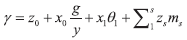 |
(1 ) ) |
In which ms represents the other control variables, which are explained at the end of the section. x0 is the coefficient that shows the effect of a change in the share of total public expenditure on output. A change in  would change the level of both types of public expenditure, as g = g1 + g2. Thus, x0 is interpreted as the effect of a change in the level of g1 and g2.
In equation (1), only θ1, the share of g1 in total public expenditure, is included, because including θ2, the share of g2 in total public expenditure, would lead to perfect collinearity, as θ1 + θ2 = 1. This also means that the coefficient of the share of g1 in total public expenditure shows the effect of a change in θ1 with respect to a change in θ2, because an increase (or a decrease) in θ1 entails a reduction (or a rise) in θ2.
The specification of the regression model becomes slightly more complicated if there are more than two types of public expenditure. If there are n types of public expenditure, then the components of public expenditure could be expressed as:
| The first type of public expenditure: |
g1 = θ1g |
| The second type of public expenditure: |
g1 = θ2g |
| The nth type of public expenditure: |
gn = θng |
g = g1 + g2 +...+ gn and θ1 + θ2 +...+ θn = 1
In this case, the regression model could be specified in two ways. The first way is to adopt equation (1), which would indirectly reduce the number of types of public
expenditure to two, as x1 would reflect the effect of a change in θ1 with respect to a change in the share of the remaining types of public expenditure (θ2 + θ3 + ... + θn). In this paper, the regression model is specified as in equation (1) for robustness of results, and simplicity in interpretation.
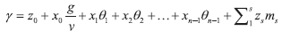
The alternative approach would be to include n – 1 types of public expenditure in the regression model, and to exclude the nth type of public expenditure to avoid perfect collinearity, as in equation (2).
| |
(2) |
However, specifying the regression model as in equation (2), firstly, complicates
the analysis, and, secondly, reduces the reliability of the results. In this case, including the shares of g2, g3, ..., gn–1 imposes the assumption that a change in θ1
impacts γ, for given values of θ2, θ3, ..., θn–1, (and  ). Thus, the coefficient of the
share of g1 in total public expenditure shows the effect of a change in θ1 with respect to a change in θn. For the same reason, the coefficients of the share of g2
(or g3,…, or gn–1) also reflect the effect of a change in θ2 (or θ3,…, or θn–1) with respect to a change in θn.
It can be seen that specifying the regression model as in equation (2) puts emphasis on the nth type of public expenditure that is left out of the equation. This complicates the analyses as the coefficient of a type of public expenditure depends on the type of public expenditure that is excluded from the model. If, for example, the regression model was specified as in equation (3), in which the share of g1 in total public expenditure is excluded, and the share of gn in total public expenditure is included in the model, the values of x2, x3, ..., xn–1 would differ from equation (2), as the coefficients would reflect the effect of a change in θ2, θ3, ..., θn–1 with respect to a change in θ1, not in θn. Considering there are n types of public expenditure, one would have to choose a regression model among n – 1 versions of equation (2). This would reduce the robustness of the results because, as the number of types of public expenditure increased, the results between equations would be more volatile, and choosing the appropriate model would be more difficult.
 |
(3) |
In Devarajan, Swaroop and Zou ( 1996), the regression models are specified as in equation (2). The authors include the shares of education, health, transportation and communication, and defence in total public expenditure in their regression models. However, they do not explain what type of public expenditure they exclude from the regression models, and, hence, it is actually not possible to interpret the full meaning of the coefficients in their paper.
In this paper, the estimated equation is defined according to equation (1) for robust analyses. Thus, the estimated model in this paper is specified as in equations (4) and (5):
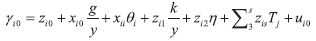 |
(4) |
where
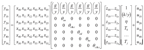 |
(5) |
and
θen + θt&c + θed + θhe + θc&s = 1
This paper applies the model in Devarajan, Swaroop and Zou ( 1996) to public investment data. Thus, in the matrix expression in equation (5), θen represents the share of energy infrastructure, θt&c, transportation and communication, θed, education, θhe, health, θc&s, city infrastructure and security, in total public investment. The other variables in the regression model in this paper are:  the share of total public investment in GDP, to control for the change in the sum of all components of public investment;  , the share of private capital in GDP in the manufacturing sector, to control for private sector investment; η, population growth rate, to control for the change in the population size in the provinces; and Tj, a dummy variable for each year in the dataset, to control for the cross-sectional fixed-effects. γ is the dependent variable, which is the five-year forward-moving geometric average of per-worker real GDP growth rate. zi0 is the constant term and ui0 is the error term.
5 Data and method
5.1 Data source
The range of the dataset in this paper is limited by the available data for GDP per province. Although data for public investment are provided for provinces up to 2017, GDP series are available for provinces only for the years 1975-2001. The dana for GDP were not reported for provinces for the years before 1975 and after 2001.
Public investment data used in this paper are taken from the State Planning Organisation (now, a section of the Ministry of Development) and reflect the amount of public capital expenditure financed by the central government budget. Data used in this paper exclude types of public investment that are made to multiple provinces, as they are not reported in a way that allows one to determine the proportion of public investment received by each province. The State Planning Organisation groups these types of public investment under the title “various provinces”.
The State Planning Organisation disaggregates public investment functionally as energy infrastructure (e.g. energy plants and electricity grids), transportation and communication (e.g. roads, railways, airports, postal service, telephone grids), education (e.g. schools, universities and student dormitories), health (e.g. health centres and hospitals), and city infrastructure and security services (e.g. piped water networks, sewage systems and security stations). Data are deflated for the base year 1987 using public investment deflators provided by the DPT ( 2001).
Data for GDP, for the years between 1987 and 2001, are provided by the Turkish Statistical Institute. For the years between 1975 and 1986, they are available in Karaca ( 2004). Both periods of GDP data are provided as deflated series for the base year 1987. Note that Karaca ( 2004) obtains GDP data for the provinces for the years between 1979 and 1986 from Özötün ( 1988), and, for the years between 1975 and 1978, from Özötün ( 1980), the latter of which is published by the State Statistcal Institute (which later became the Turkish Statistical Institute). Karaca, given that the series before and after 1986 are calculated differently, adjusts the data for the years between 1975 and 1986. He does this by assuming that, for any given calculation method with fixed prices, the output shares of provinces should be the same. Thus, he derives the output shares of the provinces from Özötün ( 1988) and ( 1980), and multiplies them by the national GDP reported by the State Statistical Institute for the years between 1975 and 1986.
Nevertheless, the consistency of the series provided by Karaca ( 2004), for the years between 1975 and 1986, and the Turkish Statistical Institute, for the years between 1987 and 2001, are checked, firstly, by calculating GDP growth rate for Turkey for the years between 1975 and 2001. Then, they are plotted against dana for Turkey’s GDP growth rate obtained from the World Bank ( 2017) for the years between 1975 and 2001. The annual growth rates calculated from data series used in this paper do not differ from those provided by the World Bank, which is an indication that the GDP series taken from Karaca ( 2004) and the Turkish Statistical Institute are consistent 4.
Data for private capital include gross investments in fixed capital in the manufacturing sector. The data are collected by annual manufacturing sector surveys carried out by the Turkish Statistical Institute. This indicator is included in the regression to capture the impact of private capital on economic growth. As it measures private investment only in the manufacturing sector, it also reflects the level of industrialisation in the provinces. Data for private capital are deflated for the year 1987 using the deflator series for the manufacturing sector in DPT ( 2001).
The population growth rate is included in the regressions because it is one of the determinants of the size of the workforce, which has an effect on the denominator of GDP per worker. The population growth rate is calculated using the census statistics. Census statistics were collected in 1975, 1980, 1985, 1990 and 2000 by the Turkish Statistical Institute. The population growth rate reflects the annual growth in the number of people between census years. It is computed by the formula,  in which Nt is the size of population in census year t and Nt+h is the size of population in census year t + h. For example, for 1978, the population growth rate equals  while for 1998, the population growth rate is  .
It must be noted that the data for the population growth rate are problematic by construction as they remain fixed between census years. Nevertheless, the variable is retained in the regressions for two reasons: firstly, the population growth rate is a key demographic indicator, the exclusion of which could lead to omitted variable bias. Secondly, the Hausman test for model specification in the post-estimation diagnostics suggests using the random-effects and the pooled OLS techniques, both of which render the population growth rate a useful indicator as it changes considerably from province to province due to domestic migration, despite its shortcomings in terms of reflecting the change in population within panels.
In this paper, the economic growth rate is calculated using data for real GDP per worker. For the denominator, the data for the number of workers are also taken from census data collected in 1975, 1980, 1985, 1990 and 2000. The number of workers for in-between census years is calculated by assuming the size of the workforce would increase at a fixed annual growth rate. Thus, the number of workers for year t + 1 is obtained using the formula,  in which Lt is the number of workers in census year t, and Lt+j is the number of workers in census year t+ j. The intervals in census data and the computation of the size of the workforce impose disadvantages on the denominator of GDP per worker similar to those discussed in relation to the population growth rate.
In the empirical analysis, public investment in year t is expected to impact the growth rates between years t + 1 and t + 5. Thus, the dependent variable is defined as the five-year forward-moving geometric average of per-worker real GDP growth rate using the formula,  The reason for using the five-year forward-moving geometric average of per-worker real GDP growth rate is discussed in more detail in the next section.
5.2 Econometric method
For the econometric analysis of the relationship between the composition of public investment and economic growth, this paper benefits from the empirical practices applied in the research regarding the link between public expenditure and economic growth. One of the major problems in estimating the effect of public expenditure on economic growth is reverse causality, which implies that public expenditure might be endogenous as an explanatory variable in regressions. Reverse causality arises due to the difficulty of identifying whether economic growth is a consequence of a change in public expenditure or is the cause of that change in public expenditure. In a case in which the model is static, the effect of public expenditure on economic growth rate might be a result of an increase or a decrease in output rather than a factor that explains the change in it. That is, it might be the case that, as higher economic growth is achieved, a government will spend more. The other possibility is that, as a public policy, the government, in order to promote growth, might spend more in some sectors, and the effect of this spending might not be observed if the income per capita and the relevant spending are contemporaneous. These are issues that might affect the robustness of results in this paper too.
The econometric problem is that if public expenditure were endogenous to the system, ordinary least squares (OLS) estimates would be biased and inconsistent, because the assumption that the error term and explanatory variables are uncorrelated would be violated. In the literature, there are two common methods to address the problem of simultaneous endogeneity of public expenditure. Some researchers (Bose, Haque and Osborn, 2007; Chamorro-Narvaez, 2012; Ghosh and Gregoriou, 2008) prefer to apply dynamic panel data estimation techniques that are derived from the generalised method of moments (GMM), which allows them to use the lagged values of dependent or explanatory variables as instruments.
Others (Devarajan, Swaroop and Zou, 1996; Haque, 2004; Odedokun, 2001) specify the dependent variable as the five-year forward-moving average of per-capita GDP growth rate to address the possibility of reverse causality. Both of these approaches are applicable in the empirical analysis of the relationship between public investment and economic growth.
The advantage of the GMM is that it is a technique developed specifically for the problem of endogeneity. The method introduced by Arellano and Bond ( 1991) has small sample bias; in other words, the technique requires the time dimension of the dataset to be sufficiently large. Later, this weakness was addressed by Arellano and Bover ( 1995), and Blundell and Bond ( 1998 ), and the system GMM estimator was proposed. However, these techniques require error terms to be uncorrelated between panels (Stata, 2017a; 2017b). Because this paper uses a dataset that consists of provinces and, as the workforce and capital are more fluid between provinces than between countries, the error terms are likely to be correlated between provinces, which violates this assumption 5.
Thus, in this paper, to address endogenous simultaneity, the second approach is preferred. It requires calculating the dependent variable as the n-year forwardmoving average of the growth rate. This introduces serial correlation to standard errors within panels which can be corrected using relevant statistical methods 6. The problem of reverse causality is addressed by avoiding using the contemporaneous values of public expenditure and economic growth rate in the regression. While, as the explanatory variable, the value of public expenditure in year t is used, as the dependent variable, the growth rate in year t + 1 is taken into consideration. To account for the impact of public expenditure on future growth rates, the dependent variable is calculated as the n-year forward-moving average of the growth rate, which is the average of the growth rates between t + 1 and t + n. This paper adopts this approach for public investment.
Following the empirical literature (Devarajan, Swaroop and Zou, 1996; Haque, 2004; Odedokun, 2001), this paper uses the five-year forward-moving average of the growth rate as the dependent variable. However, this paper differs from the cited papers in two aspects. Instead of computing the dependent variable as the nomic growth rate. This is because the geometric average is more reliable than the arithmetic average, as the growth rate is a variable that fluctuates considerably. Secondly, this paper prefers using data for real GDP per worker instead of real GDP per capita, to account for the changes in the size of the workforce in output production 7.
In this paper, the results obtained from the random-effects and pooled OLS techniques are reported. In panel data analysis, there are two main causes of concern: spatial and temporal dependence. If these lead to dependence between error terms, the inferential statistics become biased. If they are common factors that are correlated with the explanatory variables, their omission leads to biased coefficients. To address temporal dependence, the within-estimator that subtracts the individual effects that are fixed over time is used, while, to address spatial dependence, the between-effects estimator that eliminates the individual effects that are constant across the cross-sections (space) is required. The random-effects estimator is the equally weighted average of the within and between estimators. It allows for spatial dependence between error terms but assumes that it is not a common factor that is correlated with the explanatory variables. Meanwhile, the pooled OLS estimator assumes the observations are independent.
To choose between the econometric techniques, two diagnostic tests are commonly used as indicators. To check whether spatial or temporal dependence is a common factor that is correlated with the explanatory variables, the Hausman test for model specification is applied. To control for the spatial dependence between error terms, the Breusch and Pagan Lagrangian multiplier test is used. In this paper, the post-estimation diagnostics show that the Hausman test for model specification fails to reject the null hypothesis that there is not a systematic difference between the coefficients produced by the fixed-effects and random-effects techniques, or the fixed-effects and pooled OLS techniques. This also means that the between-effects and fixed-effects estimators are equivalent, in other words, the results would not differ between the spatial and temporal panel data techniques 8. In the lack of spatial and temporal dependence, the random-effects and pooled OLS techniques are considered more efficient. Thus, in this paper, these techniques are preferred over the fixed-effects (or the between-effects) technique.
Breusch and Pagan Lagrangian multiplier test indicates spatial dependence in error terms, which leads to serial correlation in residuals between panels and, thus, biased inferential statistics. This requires choosing the random-effects estimator over the pooled OLS estimator because the former is derived from the generalised least squares technique which allows for spatial dependence in error terms. However, this problem can also be addressed by using a correction technique for standard errors that clusters the observations. Therefore, for the results obtained from the pooled OLS technique, standard errors robust to heteroscedasticity, and serial correlation within panels (temporal autocorrelation) and between panels (spatial autocorrelation) are reported, while, for the results estimated by the randomeffects technique, standard errors robust to heteroscedasticity and serial correlation within panels are presented.
As a final note, it must be added that, although the Hausman test for model specification provides evidence regarding the robustness of the coefficients, and despite correcting the standard errors to address the presence of cross-sectional autocorrelation in residuals as indicated by the Breusch and Pagan Lagrangian multiplier test, spatial dependence remains an issue that can affect the robustness of the results in this paper.
6 Results and discussions
6.1 Descriptive statistics
Summary statistics are provided in table 1. The number of observations (N) in the sample is 1407. The sample is divided into 67 panels (n) that contain 22 years (T). The number of observations in the original dataset for public investment indicators is 1809. The dataset consists of 67 panels (n) and 27 (T) years. However, the size of the dataset reduces when the dependent variable is calculated as the fiveyear forward-moving geometric average of per-worker real GDP growth rate. This is because real GDP per worker is available only for the years between 1975 and 2001. Thus, calculating the value of the dependent variable for 1997, 1998, 1999, 2000 and 2001 is not possible, as this requires the values of real GDP per worker for 2002 and onwards. Nevertheless, the length of the dataset is considered to be the years between 1975 and 2001, as the five-year forward-moving geometric average of per-worker real GDP growth rate, even if indirectly, reflects the changes in output per worker between these years.
Turkey experienced many economic crises between the years 1975 and 2001; thus, on average, the five-year forward-moving geometric average of per-worker real GDP growth rate is low (1.8%) for a developing country. For the same reason, the size of the standard deviation of the dependent variable within panels is rather high. The value of an observation deviates from the sample mean by 3.2%, which is nearly twice as high as the sample mean. The size of the standard deviation between panels indicates that the five-year forward-moving geometric average of per-worker real GDP growth rate varies significantly across the provinces as well. This is due to the disparity in the level of economic development across the provinces in Turkey.
The minimum and maximum values of the dependent variable across observations, between panels and within panels, provide examples of extreme cases. The highest value of the five-year forward-moving geometric average of per-worker real GDP growth rate is observed in Adiyaman in 1986, which is 17.8%. 9 The minimum value of the dependent variable across observations is -9.1%, which is observed in Mus in 1982. This is likely to be related to the economic crisis between 1978 and 1981, which may have affected the growth rates reported in Mus in the following years.
Average shares of the components of public investment for the estimated sample can be ordered by magnitude of the values from highest to lowest as city infrastructure and security services (30.0%), energy infrastructure (26.7%), education (21.6%), transportation and communication (14.8%), and health (6.9%). Overall minimum values show that the shares of transportation and communication, education and health in total public investment are zero. This is because some provinces do not receive public investment in some sectors. Similarly, overall maximum values of the shares in total public investment are over 90%. This is because some provinces in the sample receive public investment only in one sector, such as in energy, or transportation and communication. The values of the overall standard deviations of the components of public investment are very high with respect to the mean of the variables. This indicates high variation in public investment across regions and time.
The summary statistics for the share of total public investment in GDP are in accordance with the summary statistics for the components of public investment. The share of total public investment in GDP is 3.7% on average. The maximum value for the overall observations is 87.3%. This is due to provinces (such as Bingol, Kahramanmaras and Sanliurfa) that are underdeveloped. Their economies are so minuscule that the level of their GDP is hardly above the value of the public investment they receive.
The average of the population growth rate in the dataset is 1.6%. The statistics show that the value of population growth rate is negative for some provinces, and it can be as low as -3.5%. This is a result of domestic migration, which leads to negative population growth rates for the provinces from which people emigrate. Migration also makes the rate of population growth considerably higher in those provinces that receive domestic migrants. The maximum value of the overall sample is 10.1%. The minimum value of the panel means shows that some provinces consistently had a negative population growth rate in the sample.
Summary statistics show that the average share of private capital in GDP for Turkey in the estimated sample is 1.3%. The values of standard deviation show that it varies both between and within provinces by 1.9%. This is further evidence for disparity in the level of development across provinces. Its value is negative for some provinces (Diyarbakır, Isparta, Niğde and Sinop) for the years that coincide with the economic crises the country experienced (such as between 1984 and 1986, and between 1994 and 1996). Additionally, its value is zero for some provinces (such as Adiyaman, Agri and Hakkari) that are underdeveloped and rural.
The pairwise correlation matrix for the variables can be found in table 2. Overall statistics show that the values of correlation coefficients are below 20%. However, the public investment indicators appear to be correlated with each other. It should be added that they are included in the regressions separately; thus, multicollinearity is unlikely to be an issue in the results. Nevertheless, the values of the correlation coefficients between the share of total public investment in GDP and the shares of energy infrastructure, education, and city infrastructure and security in total public investment are over 30%, which is a factor that reduces the reliability of the results. Considering this, in the next section, the values of the variance inflation factors are also reported to establish the robustness of the results to collinearity between the variables.
Table 1Descriptive statistics DISPLAY Table
Table 2Pairwise correlation matrix for the variables DISPLAY Table
6.2 Regression analysis
The results are reported in tables 3 and 4. In table 3, the results are obtained from the random-effects technique with standard errors robust to heteroscedasticity and serial correlation within panels. In table 4, the results obtained from the pooled OLS with standard errors robust to heteroscedasticity, serial correlation within and between panels are reported.
The results in table 3, firstly show that the coefficients of the shares of energy infrastructure, health, education, and city infrastructure and security services in total public investment are not statistically significant. It appears that the coefficient of the share of transportation and communication in total public investment is negative and statistically significant in the third column. The share of total public investment in GDP has a positive and statistically significant coefficient in all columns. The coefficient of the population growth rate is not statistically significant in any of the regressions. The share of private capital (in the manufacturing sector) in GDP has a positive and statistically significant coefficient in the overall results. In table 4, the results remain similar to those in table 3, except for the coefficient of the share of energy infrastructure in total public investment, which becomes statistically significant with a positive sign.
In tables 3 and 4, Wald χ2 and F statistics indicate the coefficients of the variables in the regressions are jointly statistically significant. The values of R2 show that the variables explain 17 to 18% of the change in the dependent variable. The average values of the variance inflation factors (mean VIF) for the regressions in tables 3 and 4 provide evidence that the results are robust to multicollinearity.
Overall results suggest that, if the share of total public investment in GDP and other factors are held constant, shifting the public investment from transportation and communication to other sectors contributes positively to the five-year forward-moving geometric average of per-worker real GDP growth rate. Shifting 1% of the public investment from transportation and communication to other sectors is associated with an increase that is between 0.016% and 0.019% in the dependent variable. Devarajan, Swaroop and Zou’s ( 1996) model above indicates that public policy overinvested in transportation and communication services in the years between 1975 and 2001. The results in table 4 appear to indicate that, among public investment in education, health, city infrastructure and security, and energy infrastructure, it is the latter in which there has been underinvestment.
It must be noted that, given the economic model discussed in the previous section, the results do not provide information as to whether a particular type of public investment is more or less productive than another. They simply indicate the allocation of public investment between transportation and communication, energy infrastructure, education, health, and city infrastructure and security is not optimum. Although investment in transportation and communication might be productive per se, results indicate that other public investment layouts would yield higher output for a unit increase in the amount of resources.
According to Devarajan, Swaroop and Zou’s ( 1996) model, the government does not need to increase the level of overall public investment to increase the growth rate. Public policy can achieve a higher growth rate simply by shifting resources from transportation and communication layout to other types of public investment. The results in table 4 imply that, ideally, this should be public energy infrastructure.
The results also indicate that the level of public investment is positively related to the five-year forward-moving geometric average of per-worker real GDP growth rate. For a given public investment composition, increasing the share of total public investment in GDP is associated with higher values of the dependent variable. Findings regarding the coefficient of the level of public investment are consistent with the implication of the economic model presented in this paper. The Devarajan, Swaroop and Zou ( 1996) model suggests that, even though the coefficient of the share of transportation and communication in total public investment is negative, this does not mean that investment in this layout is unproductive per se. The positive coefficient of the level of public investment supports this point and suggests that, even though the resources are misallocated among the public investment layouts, if there were no budget constraints, increasing their amount would have a positive growth effect.
Statistical evidence in this paper indicates that returns to public capital are slightly lower than the returns to private capital. While a 1% increase in the share of total public investment in GDP is associated with a 0.05 to 0.09% increase in the five-year forward-moving geometric average of per-worker real GDP growth rate, a 1% increase in the share of private capital in GDP in the manufacturing sector is related to a 0.10 to 0.16% increase in the dependent variable. The results are in agreement with Khan and Kumar ( 1997), who find that the rate of return for public capital is 0.29%, while the rate of return to private investment is 0.4% for the years 1970-1990 for a cross-section of developing countries. Their results also indicate that the productivity of private capital is higher than that of public capital.
The population growth rate does not appear to be related to the five-year forward-moving geometric average of per-worker real GDP growth rate. Becker, Glaeser and Murphy ( 1999) show that, although the effect of population becomes negative as land and other natural resources have diminishing returns, it can also be a source of growth through its positive impact on human capital. The results appear to imply that the negative and positive effects of population movements between provinces cancel each other out.
It should be added that the statistical significance of the coefficient of the share of transportation and communication in total public investment in table 4 is robust to alternative specification of the dependent variable, such as the ten-year or the fifteen-year forward-moving geometric average of per-worker real GDP growth rate. This is the case if the dependent variable is calculated as the five-year forward-moving arithmetic average of per-capita or per-worker real GDP growth rate, or geometric average of per-capita real GDP growth rate. The statistical significance of the share of transportation and communication in total public investment in table 3, although robust to using wider time spans in computation of the dependent variable, is sensitive to the specification of the dependent variable in per capita terms or calculating it as an arithmetic average 10.
For the five-year forward-moving geometric average of per-worker real GDP growth rate, the coefficient of the share of transportation and communication in total public investment in tables 3 and 4 becomes statistically insignificant when the fixed-effects technique is used. However, for wider time spans of the dependent variable, its coefficient becomes statistically significant according to the fixedeffects technique too.
The statistical significance of the share of total public investment in GDP in tables 3 and 4 is robust to both alternative specifications of the dependent variable and using the fixed-effects as the econometric technique. However, the statistical significance of the coefficient of the share of private capital in GDP depends on the computation of the dependent variable and the chosen econometric technique. This appears to be the case for the population growth rate too, which becomes statistically significant for the ten-year or the fifteen-year forward-moving geometric average of per-worker real GDP growth rate 11.
Table 3Composition of public investment and economic growth: random-effects technique-standard errors corrected for heteroscedasticity and serial correlation DISPLAY Table
Table 4Composition of public investment and economic growth: pooled OLS technique-standard errors corrected for heteroscedasticity, and serial correlation both within and between panels DISPLAY Table
7 Conclusion and limitations
In this paper, the relationship between the composition of public investment and economic growth has been analysed. According to the model used in the paper, results indicate that, for the years between 1975 and 2001, public policy led to an overinvestment in transportation and communication services. As the GDP dana for the provinces after 2001 are not reported by the Turkish Statistical Institute, it is not possible to draw a policy implication regarding the country’s more current economic climate. Results in this paper only indicate that the misallocation of public resources is likely to have led to sub-optimum growth rates between 1975 and 2001. Nevertheless, this paper provides an approach to the assessment of public policy that could be applied to data for the years after 2001 if the GDP series for the provinces were made available by the Turkish Statistical Institute.
Devarajan, Swaroop and Zou ( 1996) provide a useful analytical tool that helps to identify whether the distribution of public resources between infrastructure, education and health is optimum. The strength of their model is the lack of restrictions regarding the productivity of public investment layouts. However, this is also the model’s weakness, as it does not provide any insight into the reasons for the misallocation of resources. Thus, the model does not explain why it is the transportation and communication services that are overinvested in. Is it because investment in this sector is less productive in general or because the amount of spending in this layout too high? It is not possible to answer these questions using the economic model presented in this paper.
The second limitation of this paper is the assumption that there is no reverse causality between the dependent variable and public investment indicators. To reduce the possibility of the endogeneity of the public policy in determining the amount of public investment, the dependent variable is calculated as the five-year forwardmoving geometric average of per-worker real GDP growth rate. Nevertheless, public policy might be impacted by the expected future growth rates, which would lead to biased results.
Notes
* The author would like to thank to two anonymous referees for useful comments and suggestions.
1 Public investment corresponds to public capital expenditure. This paper adopts the former term whenever it refers to its sample. This is because the State Planning Organisation (now, a section of the Ministry of Development) reports these data under the title “public investment”).
2 Note that, with the real GDP data for the years between 1975 and 2001, the dependent variable can be calculated for the years between 1975 and 1996.
3 Available on request.
4 The figure is provided as part of the post-estimation diagnostics on request.
5 The post-estimation diagnostics show the presence of serial correlation in residuals both within and between panels.
6 Deverajan, Swaroop and Zou (1996) and Haque (2004) correct the standard errors using the methodology in Hansen and Hodrick (1980). This paper uses the built-in commands in the statistical software (Stata) used for the empirical analysis of the data. For panel data, the command “xtreg” offers the “robust” option which corrects the standard errors to heteroscedasticity and serial correlation, while the command “xtscc” allows for correcting the standard errors to heteroscedasticity and serial correlation between panels, and within panels up to a specific number of lags. In this paper, the standard errors obtained from the “xtscc” command are corrected for serial correlation within panels up to five lags, as the five-year forward-moving geometric average of per-worker real GDP growth rate introduces correlation to error terms between years t and t+5 (Devarajan, Swaroop and Zou, 1996). Note that, while the command “xtreg” offers the random-effects and fixed-effects techniques, the command “xtscc” offers pooled OLS and fixed-effects techniques as econometric methods. In accordance with the results of the Hausman test for model specification in the post-estimation diagnostics, Table 3 uses the random-effects technique, while Table 4 uses the pooled OLS technique.
7 Robustness of the results to alternative specification of the dependent variable is discussed in the end of the results section.
8 This, indeed, appears to be the case, as the results remain similar if one uses the between-effects estimator provided by the statistical software Stata.
9 The dataset has been examined for errors in data entry and the calculation of the dependent variable but neither of these appears to be the case.
10 Between tables 3 and 4, the statistical significance of the coefficient of the share of energy infrastructure in total public investment is sensitive to the treatment of residuals for heteroscedasticity, and serial correlation between and within panels. For this reason, the robustness analysis regarding alternative specifications of the dependent variable focuses on the share of transportation and communication in total public investment, which is the only public investment component that has a statistically significant coefficient in both Table 3 and Table 4.
11 All the results are available on request.
* The author would like to thank to two anonymous referees for useful comments and suggestions.
1 Public investment corresponds to public capital expenditure. This paper adopts the former term whenever it refers to its sample. This is because the State Planning Organisation (now, a section of the Ministry of Development) reports these data under the title “public investment”).
2 Note that, with the real GDP data for the years between 1975 and 2001, the dependent variable can be calculated for the years between 1975 and 1996.
4 The figure is provided as part of the post-estimation diagnostics on request.
5 The post-estimation diagnostics show the presence of serial correlation in residuals both within and between panels.
6 Deverajan, Swaroop and Zou ( 1996) and Haque ( 2004) correct the standard errors using the methodology in Hansen and Hodrick ( 1980). This paper uses the built-in commands in the statistical software (Stata) used for the empirical analysis of the data. For panel data, the command “xtreg” offers the “robust” option which corrects the standard errors to heteroscedasticity and serial correlation, while the command “xtscc” allows for correcting the standard errors to heteroscedasticity and serial correlation between panels, and within panels up to a specific number of lags. In this paper, the standard errors obtained from the “xtscc” command are corrected for serial correlation within panels up to five lags, as the five-year forward-moving geometric average of per-worker real GDP growth rate introduces correlation to error terms between years t and t+5 (Devarajan, Swaroop and Zou, 1996). Note that, while the command “xtreg” offers the random-effects and fixed-effects techniques, the command “xtscc” offers pooled OLS and fixed-effects techniques as econometric methods. In accordance with the results of the Hausman test for model specification in the post-estimation diagnostics, Table 3 uses the random-effects technique, while Table 4 uses the pooled OLS technique.
7 Robustness of the results to alternative specification of the dependent variable is discussed in the end of the results section.
8 This, indeed, appears to be the case, as the results remain similar if one uses the between-effects estimator provided by the statistical software Stata.
9 The dataset has been examined for errors in data entry and the calculation of the dependent variable but neither of these appears to be the case.
10 Between tables 3 and 4, the statistical significance of the coefficient of the share of energy infrastructure in total public investment is sensitive to the treatment of residuals for heteroscedasticity, and serial correlation between and within panels. For this reason, the robustness analysis regarding alternative specifications of the dependent variable focuses on the share of transportation and communication in total public investment, which is the only public investment component that has a statistically significant coefficient in both Table 3 and Table 4.
11 All the results are available on request.
Disclosure statement
No potential conflict of interest was reported by the author.
References
Afonso, A. and Furceri, D., 2010. Government Size, Composition, Volatility and Economic Growth. European Journal of Political Economy, 26(4), pp. 517–532. [ CrossRef]
Agénor, P. R. and Moreno-Dodson, B., 2006. Public Infrastructure and Growth: New Channels and Policy Implications. Policy Research Working Paper Series [ CrossRef]
Agénor, P. R. and Neanidis, K. C., 2011. The Allocation of Public Expenditure and Economic Growth. The Manchester School, 79(4), pp. 899–931. [ CrossRef]
Agénor, P. R., 2009. Infrastructure Investment and Maintenance Expenditure: Optimal Allocation Rules in a Growing Economy. Journal of Public Economic Theory, 11, pp. 233–250 [ CrossRef]
Arellano, M. and Bond, S., 1991. Some Tests of Specification for Panel Data: Monte Carlo Evidence and an Application to Employment Equations. The Review of Economic Studies, 58(2), pp. 277–297 [ CrossRef]
Arellano, M. and Bover, O., 1995. Another Look at the Instrumental Variable Estimation of Error-Components Models. Journal of Econometrics, 68(1), pp. 29–51 [ CrossRef]
Aschauer, D. A., 1989. Is Public Expenditure Productive? Journal of Monetary Economics, 23(2), pp. 177–200.
Barro, R. J. and Sala-I-Martin, X., 1992. Public Finance in Models of Economic Growth. The Review of Economic Studies, 59(4), pp. 645–661 [ CrossRef]
Becker, G. S., Glaeser, E. L. and Murphy, K. M., 1999. Population and Economic Growth. American Economic Review, 89(2), pp. 145–149 [ CrossRef]
Blundell, R. and Bond, S., 1998. Initial Conditions and Moment Restrictions in Dynamic Panel Data Models. Journal of Econometrics, 87(1), pp. 115–143 [ CrossRef]
Bose, N., Haque, M. E. and Osborn, D. R., 2007. Public Expenditure and Economic Growth: A Disaggregated Analysis for Developing Countries. The Manchester School, 75(5), pp. 533–556 [ CrossRef]
Chamorro-Narvaez, R. A., 2012. The Composition of Government Spending and Economic Growth in Developing Countries: The Case of Latin America. OIDA International Journal of Sustainable Development, 5, pp. 39–50.
Chen, B., 2006. Economic Growth with an Optimal Public Spending Composition. Oxford Economic Papers, 58(1), pp. 123–136 [ CrossRef]
Devarajan, S., Swaroop, V. and Zou, H., 1996. The Composition of Public Expenditure and Economic Growth. Journal of Monetary Economics, 37(2), pp. 313–344 [ CrossRef]
Easterly, W. and Rebelo, S., 1993. Fiscal Policy and Economic Growth. Journal of Monetary Economics, 32(3), pp. 417–45 [ CrossRef]
Ghosh, S. and Gregoriou, A., 2008. The Composition of Government Spending and Growth: Is Current or Capital Spending Better? Oxford Economic Papers, 60(3), pp. 484–516 [ CrossRef]
Gupta, S. [et al.], 2005. Fiscal Policy, Expenditure Composition, and Growth in Low-Income Countries. Journal of International Money and Finance, 24(3), pp. 441–463 [ CrossRef]
Hansen, L. and Hodrick, R., 1980. Forward Exchange Rates as Optimal Predictors of Future Spot Rates: An Econometric Analysis. Journal of Political Economy, 88(5), pp. 829–53 [ CrossRef]
Haque, M. E., 2004. The Composition of Public Expenditures and Economic Growth in Developing Countries. Global Journal of Finance and Economics, 1(1), pp. 97–117.
Karaca, O., 2004. Turkiye’de Bolgeler Arasi Gelir Farkliliklari: Yakinsama Var mi? Tartisma Metni, No. 7.
Khan, M. S. and Kumar, M. S., 1997. Public and Private Investment and the Growth Process in Developing Countries. Oxford Bulletin of Economics and Statistics, 59(1), pp. 69–88 [ CrossRef]
Lee, J., 1992. Optimal Size and Composition of Government Spending. Journal of the Japanese and International Economies, 6(4), pp. 423–439 [ CrossRef]
León-González, R. and Montolio, D., 2004. Growth, Convergence and Public Investment: A Bayesian Model Averaging Approach. Applied Economics, 36(17), pp. 1925–1936 [ CrossRef]
Özötün, E., 1980. İller İtibariyle Türkiye Gayri Safi Yurtiçi Hasılası-Kaynak ve Yöntemler, 1975-1978. Ankara: Devlet İstatistik Enstitüsü.
Özötün, E., 1988. Türkiye Gayri Safi Yurtiçi Hasılasının İller İtibariyle Dağılımı, 1979-1986. İstanbul: İstanbul Ticaret Odası Araştırma Bölümü.
Pereira, A. M. and Andraz, J. M., 2005. Public Investment in Transportation Infrastructure and Economic Performance in Portugal. Review of Development Economics, 9(2), pp. 177–196 [ CrossRef]
Ramirez, M. D. and Nazmi, N., 2003. Public Investment and Economic Growth in Latin America: An Empirical Test. Review of Development Economics, 7(1), pp. 115–126 [ CrossRef]
Shioji, E., 2001. Public Capital and Economic Growth: A Convergence Approach. Journal of Economic Growth, 6(3), pp. 205–227 [ CrossRef]
Turnovsky, S. J. and Fisher, W. H., 1995. The Composition of Government Expenditure and Its Consequences for Macroeconomic Performance. Journal of Economic Dynamics and Control, 19(4), pp. 747–786 [ CrossRef]
DATA SOURCE
Public Investment Kutbay, C. 1982. Kamu Yatırımlarının Kalkınmada Öncelikli İller İtibariyle Dağılımı: 1963-1981, No. 1830, Ankara: DPT Yayınları. DPT, 1975-2001. Kamu Yatırımlarının İllere Göre Dağılımı
Public Investment Deflators DPT, 2002. Yatırım Programı Hazırlama Esasları.
Population 1980: DİE 1983 Genel Nüfus Sayımı Nüfusun Sosyal ve Ekonomik Nitelikleri 12.10.1980 Census of Population Social and Economic Characteristics of Population 1975: DİE 1982 Genel Nüfus Sayımı Nüfusun Sosyal ve Ekonomik Nitelikleri 26.10.1975 Census of Population Social and Economic Characteristics of Population
Capital Stock in the Manufacturing Sector DİE, 1978-2004. Yıllık İmalat Sanayi İstatistikleri, Annual Manufacturing Industry Statistics
Gross Domestic Product
|


