|
|
|
Abstract
The aim of this paper is to investigate the extent to which local budget composition reacts to variations in fiscal spending rules. It looks at Italian subnational governments and specific changes in the institutional framework, implementing a difference-in-discontinuities strategy. Results show that when a reduction in current spending is imposed, local authorities direct the cuts towards services. Furthermore, when an increase in capital spending is allowed, there is an increase in spending on infrastructure and local public debt.
Keywords: fiscal rules; public spending; difference-in-discontinuities; local governments
JEL: C21, C23, H72, H74, H77
1 Introduction
Rules for coordinating the financial relationship among different government levels have the purpose of guaranteeing both macroeconomic stability and financial sustainability. Fiscal rules are generally justified because they act as a substitute for reputation when government policy is discretionary and time-inconsistent. Poterba ( 1996) compares the “institutional irrelevance view”, where budget rules can be circumvented, with the “public choice view”, where fiscal institutions represent important constraints on the behaviour of political actors, suggesting the predominance of the latter. 1996) compares the “institutional irrelevance view”, where budget rules can be circumvented, with the “public choice view”, where fiscal institutions represent important constraints on the behaviour of political actors, suggesting the predominance of the latter.
The European Stability and Growth Pact, adopted in 1997, is a set of rules designed, among other goals, to ensure sound public finances. 1 In order to be compliant with the Stability and Growth Pact, member states can implement subnational fiscal rules, imposing fiscal discipline on subnational governments. For instance, in 1999 the Italian government implemented subnational fiscal rules under the so-called Domestic Stability Pact (hereafter DSP) to coordinate and control subnational budget balances. In contrast to the attitude to national fiscal rules, there has been a controversial debate about the necessity of subnational rules. Authors such as Eichengreen and von Hagen ( 1996), Rodden ( 2002) and Rodden ( 2004) are in favour of these rules, arguing that the scope for subnational fiscal rules is higher when there are severe fiscal imbalances, possibly exacerbated by the decentralization process. In fact, when more functions are delegated to local governments, their spending power rises, and imbalances may worsen. In addition, local governments have incentives to free-ride on fiscal discipline because they can rely on a common pool of national resources (Weingast, 2009) or they are “too big to fail” (Wildasin, 1997). On the other hand, Milesi-Ferretti ( 2004) argues against subnational fiscal rules, suggesting that local rules might lead to “ugly outcomes” for local governments, such as creative accounting and window dressing. Ter-Minassian ( 2007) affirms that fiscal rules should only be implemented when finanfinancial discipline.
Fiscal rules may also be implemented to foster virtuous behaviour. Dovis and Kirpalani ( 2017) investigate whether subnational fiscal rules correct the local incentives to over-borrow, due to their expectations of bailouts by central governments. They suggest that fiscal rules can be welfare-reducing if the reputation of the central government is low enough, leading to even more debt accumulation. Debrun et al. ( 2008) suggest that certain rules, such as those targeting the budget balance or general government debt, have a significant effect on deficits, but expenditure rules do not by themselves have a significant impact on budget balances. In a survey of recent studies, Wyplosz ( 2012) finds that fiscal rules are often too easily dismissed when they are in conflict with political goals. However, Glaeser ( 2013) shows that fiscal rules at the local level are more likely to be observed than rules at the level of the national government. Poterba ( 1994) studies the dynamics of state taxes and spending during the late 1980s, pointing out that more restrictive state fiscal rules, such as “no-deficit-carryover” rules and tax and expenditure limitations, are linked to faster fiscal adjustment to unexpected deficits. Heinemann, Moessinger and Yeter ( 2018), using a meta regression analysis on 30 studies, find that there is a consensus that fiscal rules influence fiscal aggregates, particularly for deficits but less for debt, expenditures and revenues.
In relation to the compositional consequences of fiscal rules for public budgets, Foremny ( 2014) examines EU15 regional and local governments over the period 1995-2008. They suggest that subnational fiscal rules are effective in unitary countries, specifically in limiting deficits and large debts, while there is no clear evidence in federal countries, due to the larger legal fiscal autonomy. The fact that subnational fiscal rules reduce public deficits is also found by Burret and Feld ( 2018) in the case of Swiss cantons, while Bergman, Hutchison and Jensen ( 2016) show that fiscal rules foster sound public finances in a panel of EU countries. Grisorio and Prota ( 2015) study Italian regional administrations over the period 1996-2008 and show that an increase in fiscal decentralization affects public expenditure composition, specifically through a reduction in the share of capital to total expenditure.
The aim of this paper is to assess empirically the extent to which fiscal spending rules are able to affect local behaviour, and for this purpose the specific features of the DSP allows for implementing a natural-experiment strategy through a difference-in-discontinuity analysis. More specifically, this work targets two main research questions: - Are fiscal rules able to do what they are supposed to do? If the central government is able to enforce the subnational rules, the answer should be positive and not really surprising, considering that the legal design is confirmed. Nevertheless, a positive answer would support the finding that subnational fiscal rules are effective.
- Are budget items equally affected by fiscal rules? For instance, in the event of a budget cut, a local government could decide to focus the budget reduction not on all budget expenses proportionally, but only on specific items.
The Italian DSP has already attracted the attention of different authors. Patrizii, Rapallini and Zito ( 2006) addressed the ability of subnational governments to meet the DSP requirements, whereas Brugnano and Rapallini ( 2009) evaluate the effects of the DSP on local public borrowing requirements from 1999 to 2005. Bartolini and Santolini ( 2009) conduct a panel data analysis on the current expenditures of 246 Italian municipalities to capture the impact of the DSP, showing that the introduction of the DSP significantly reduces the level of public spending. Other authors focus on the impact of fiscal rules on the ability of local administrations to achieve fiscal discipline and sustainability. In particular, Balduzzi and Grembi ( 2011) check whether the adoption of fiscal rules has been accompanied by an increase in window dressing as measured through the level of budget fiscal residuals, without finding a variation in the level of budget residuals connected to the adoption of the DSP. Grembi, Nannicini and Troiano ( 2016) analyse Italian municipalities between 1999 and 2004, implementing a difference-in-discontinuities approach. They show highlight that relaxing fiscal rules increases deficits and lowers taxes, generating a deficit bias from zero to 2% of the total budget. This variation is mainly driven by adjustment on the revenue side.
The contribution of this paper is twofold, underlined by the two research questions. Firstly, in relation to the first question and in line with the literature on the effectiveness of fiscal rules, it confirms that fiscal rules are effective. In particular, there is evidence that when fiscal rules that impose a reduction in consumption and an increase in investment simultaneously, budget expenses react accordingly.
In relation to the second question, results show that: (a) when the fiscal rule imposes a reduction in current spending, not all items are equally affected and the most penalized is spending on services. This evidence shows that current spending is composed of different items, and a general rule that imposes a drop in spending may affect only a specific subcategory. Therefore, policy-makers may consider not targeting current spending with fiscal rules in general, but specific subcategories of current spending in a case in which a certain behaviour from local government is required. For instance, the central government could induce local authorities to decrease current spending by lowering wage expenses, while maintaining the service levels and keeping expenditures constant; (b) when the fiscal rule allows for an increase in capital spending, there actually is an increase in spending on infrastructure and in local public debt. This result is not surprising because of the so-called “golden rule”, which states that debt can be used to finance only investment. The link between an increase in investment and debt is therefore not surprising. However, the increase in public debt could be an unwanted outcome that goes beyond the initial willingness of the policy-maker, which possibly aimed to decrease current spending in favour of capital spending, but without the intention to increase public debt. In this case, the policy-maker could design fiscal rules that directly target subcategories of budget items able to foster the desired local behaviour, possibly also limiting the use of debt to finance investment.
As the focus is mainly on economic explanatory variables, this study is not related to the vast amount of political economy research on local public finance.
The remainder of this paper is organised as follows. Section 2 analyses the normative framework of local Italian budget rules, while section 3 focuses on the theoretical background. Section 4 illustrates the empirical analysis and results and section 5 concludes.
2 Normative framework and preliminary evidence
Italian municipalities are subject to the Law for Local Authorities,2 in which the goals and duties of local government are stated. Moreover, starting from 1999, the central government imposed the DSP to honour commitments taken with European Institutions.3
Since its introduction, the DSP has implemented different types of rules, such as: (a) a balanced budget, whereby the total amount of revenue has to be equal to the total amount of expenditure; (b) expenditure caps, through which there might be ceilings on total current expenditure or specific expenditure items; (c) ceilings on revenue, which enable the central government to limit local authorities’ ability to increase revenue; (d) limits on the stock of debt or the issuance of new loans; (e) restrictions on the type of expenditure that can be funded by debt (the so-called “golden rule” stating that new loans can finance only capital investments); (f) indicators of the ability to service the debt.
Among Italian municipalities, the amount of consumption (current) compared to investment (capital) spending has changed over time. As shown in figure 1, the overall consumption over GDP of municipalities was 3.96% in 1990, whilst investment was 2.47%. The distance between these two types of spending decreased in the following years: in 2005, consumption and investment over GDP reached 3.32% and 3.01% respectively. However, from 2006 onwards, whilst consumption remained stable, investment constantly decreased, falling to 1.62% in 2010. 4
Figure 1Italian municipalities’ consumption, investment and total spending as a percentage of GDP DISPLAY Figure
As stated in the introduction, the Stability and Growth Pact was adopted to ensure that EU countries pursue sound public finances, also controlling public spending at both the central and local level. Different types of public spending are able to generate dissimilar effects on the economy. Ganelli and Tervala ( 2010) state that the reallocation of consumption in favour of investment spending might generate welfare gains. Acconcia, Corsetti and Simonelli ( 2014) show that in Italy local investment spending on infrastructure has a multiplier of 1.5 on impact and 1.9 in the medium term.
Consequently, there could be an incentive by the central authority to direct local spending more towards investment. Is this goal achieved through the domestic stability pact? Since its introduction, the pact has been revised yearly. In fact, the representatives of local governments bargain each year with the central government about the way in which the pact should be designed. On the one hand, there are local needs to be addressed and, on the other hand, national and macroeconomic circumstances that the central government has to address. The outcome is that since 1999 there have been many changes. During the first years, all local governments were subject to the pact, while since 2002 municipalities under a certain threshold were exempt and special rules have been applied to the autonomous provinces of Trento and Bolzano and to the special-statute regions. 5 In the first two years of its application (i.e. 1999 and 2000), the Pact required a decrease of the aggregate deficit on a current programmes basis. From 2001 to 2006, the rule targeted the budget balance, which has to be corrected from one year to the other, also imposing limits, expressed as a ceiling with respect to historical values, on the growth rate of current expenditure.
Interestingly, in 2005 and 2006 the central government devoted specific attention to local public spending through the DSP. The national government had to control the overall growth of general government spending and the Pact was modified, imposing a constraint on subnational expenditure, defined by a ceiling on the spending growth rate. Unlike in the previous period, for the first time the limit also included capital spending. Indeed, in 2005, a cap was set on total expenditures, which could not be higher than the average spending of the previous three years augmented by 11.5%. 6 In 2006, the limit on overall spending was removed, while different ceilings on current and capital expenditures were added. Consumption was penalized, because the rule imposed a cut of 6.5% on current spending, while investment could increase by 8.1%. 7 Before, the main target rule was based on the fiscal gap, 8 while from 2007 the main constraint was on a target balance calculated on both a cash and an accrual basis. 9 The number of municipalities subject to the pact has changed since the introduction of the DSP: during the first two years, all municipalities were subject to the DSP, while since 2001 those with fewer than 5,000 inhabitants have been exempt. 10
In order to study the effect of fiscal spending rules, the analysis focuses on the period 2004-2006, as summarised in table 1, comparing municipalities subject to the DSP with those that are exempt. As shown in figure 2, from 2005 to 2006, municipalities with more than 5,000 inhabitants (Group B) slightly decreased the consumption over investment ratio (from 1.75 to 1.73), while an upward trend is found for Group A (from 1.50 to 1.76). This may be due to a budget composition effect caused by the DSP.
Table 1Fiscal rules imposed by the Domestic Stability Pact on Italian municipalities DISPLAY Table
Figure 2Level of Consumption over Investment for municipalities under 5,000 inhabitants (Group A) and above (Group B) DISPLAY Figure
This normative framework provides an opportunity to study the extent to which fiscal rules can affect budget spending decisions at a local level through a natural experiment, as further detailed in the following section.
3 Theoretical background
The institutional framework analysed in section 3 shows that decisions related to the DSP are made by the central government and are therefore exogenous with respect to local dynamics. Considering that municipalities up to 5,000 inhabitants (Group A) are not subject to the DSP, they will form the control group, while the treated group includes municipalities with more than 5,000 inhabitants (Group B). The treatment is the fiscal rule variation imposed by the DSP and the cut-off is the population level at 5,000 inhabitants.
To assess the causal effect of each fiscal rule (the treatment) on the treated group, it is necessary to consider a minimum set of assumptions with which to perform the analysis (Angrist and Pischke, 2008). Potential budget outcomes Y are the variables of interest and the actual treatment D depends on the variable Z, which is equal to 1 when a municipality is assigned to the treatment, while Z= 0 when it is assigned to the control group. The potential budget outcome of municipality m at time t depends on Z and D, which can more formally be expressed as Ymt = Ym( Zt , Dt). Therefore, the outcome Ymt(1) is when the municipality is treated and Ymt(0) otherwise. The following assumptions should be considered: 1) Stable unit treatment value assumption. The potential outcomes and treatments of unit m are independent of the potential assignment, treatments and outcomes of n ≠ m. Consequently, a municipality subject to the treatment should not influence the others (no general equilibrium effects). 2) Non-zero average causal effect of Z on D. The probability of treatment must be different between the two groups. Therefore, it is required that whoever is assigned to the treatment actually gets the treatment, or at least part of the component of the treated group. In other words, some level of compliance is necessary. 3) The exclusion restriction should hold. Consequently, the assignment only affects the outcome through the treatment. 4) Monotonicity. No one does the opposite of its assignment, regardless what the assignment is. Thus, the absence of defiers is required. Specifically, a defier would be a municipality that follows the DSP rules without any formal obligation. 5) Random assignment. All municipalities have the same probability of getting the treatment.
It should be noted that assumption (5) cannot hold due to the fact that the assignment is not random, but rather conditioned to the population level. In this case, a sharp regression discontinuity design (SRDD) could be implemented, imposing the following assumptions: 6) Assignment to treatment must only depend on observable pre-intervention variables (i.e. the population level). 7) Identification of the mean treatment effect is only possible at the threshold. 8) The continuity of potential outcomes. Limits of the expected values have to be identical at the cut-off. In other words, the budget outcomes of municipalities just before and after the cut-off level should be equal.
Under these assumptions, the SRDD can be written as (Angrist and Pischke, 2008):
where Pc is the population at the cut-off level, δ represents a small number, Ym and Pm are the potential budget outcome and population of municipality m. The estimand of this nonparametric estimation strategy is the average causal effect, E[Ym(1) − Ym(0) | Pm = Pc].
However, assumption (8) raises some issues. In order to identify the causal effect at the cut-off point, any discontinuity in the relationship between the outcome of interest and the variable determining the treatment status must be fully attributable to the treatment itself. However, there is a confounding discontinuity policy at the cut-offs, due to a change in the wage level of local politicians. In fact, the two groups of municipalities guarantee different wages in relation to the population level, with a jump at 3,000 and 5,000 inhabitants (exactly at the cut-offs). As shown by Gagliarducci and Nannicini ( 2013), better-paid politicians are able to improve internal efficiency, sizing down the government. Consequently, there is a confounding policy that might alter the identification strategy. To overcome this issue, the approach described in the following subsection can be implemented.
3.1 Difference-in-discontinuities
The confounding policy that inhibits the effectiveness of the SRDD strategy is constant over the analysed period. In order to remove the constant confounding discontinuity (i.e. different wage policies among municipalities), we can combine the difference-in-difference strategy with a regression discontinuity design, implementing a difference-in-discontinuities (DiDisc) framework (Grembi, Nannicini and Troiano, 2016).11 The assumptions that should hold are as follows: 9) The confounding discontinuity needs to be time invariant. This assumption requires that the effect of wage variations on budget outcomes among groups not vary with time. 10) The interaction between the treatment and the confounding discontinuity has to be irrelevant. Therefore, different wage policies should not generate a different reaction than the fiscal rules introduced by the DSP.
Under these assumptions, there is an estimator, the DiDisc estimator  , that identifies the local treatment effect δ0: 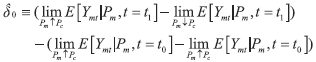 | (1 ) ) |
where Ymt is the potential budget outcome for municipality m at time t, Pm is the population level, t1 is the year of the treatment and t0 is the previous one. For each case, the assignment to the treatment is given by the dummy Dmt which takes the value:
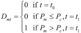 | (2) |
where Pc is the cut-off level. Having described the DiDisc strategy, we can now proceed with the empirical analysis.
4 Empirical analysis
4.1 Data
Data related to municipalities’ budgets and population levels are obtained from the Ministry of the Interior website. Budget values refer to year 2004, 2005 and 2006, deflated by the inflation considering 2006 as the reference year, and divided by the population of each municipality to obtain per-capita values. All the budget values represent the accrual basis of accounting. Municipalities in provinces and regions with “special autonomy” cannot be included in the analysis. In fact, subnational governments with “special autonomy” have the power to bargain fiscal rules directly with the Central Government. Consequently, municipalities of the autonomous provinces of Trento and Bolzano and the autonomous regions of Sicily, Sardinia, Aosta Valley, Trentino-Alto-Adige and Friuli-Venezia-Giulia are excluded from the sample. Presumably, small and large municipalities might exhibit different behaviours in terms of budget policies and therefore a specific distance from the cut-off level (5,000 inhabitants, as detailed in the next subsection) is imposed (d = 2,000).12 Consequently, the municipalities included are those between 3,000 and 7,000 inhabitants. Summary statistics are reported in table 2.
Table 2Descriptive statistics. Budget items used in the analysis by group, average of the period 2004-2006 (euro per capita) DISPLAY Table
4.2 Econometric model
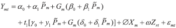
The “local linear regression” (LLR) model may be used to estimate the DiDisc estimator, as suggested by Imbens and Lemieux (2008), which fits the data with linear regression functions in a specific sample range. The interval is limited, considering a distance d from the cut-off point, thus Pm ∈ [Pc − d; Pc + d] . The estimated model is:
 | (3) |
where Ymt is the budget outcome for municipality m at time t, is the normalized population size,  is the normalized population size, with  , G being a dummy equal to 1 when a municipality is part of the treated group and 0 otherwise, t1 is the treatment year. X is a vector of time-invariant controls (i.e. area size, sea level and geographical macroarea) and Z is a vector of time-variant controls (i.e. per-capita GDP, inflation and unemployment) at the regional level r. 13 ∅ and ω are the coefficients related to the controls, while α0 is the intercept and ε is the error term. 14
The assignment to the treatment is given by the dummy Dmt = Gmt1, as explained in the previous subsection.
4.3 Results
Table 3 shows the main results, where the local treatment effects δ0 are reported for the relevant budget items.
Case A shows no effects due to the variation in the fiscal rule from budget balance to total expenditure cap. The latter rule does not affect budget composition (columns 1-3), as expected. In fact, considering that this rule allows for an increase in the overall spending, a difference in the budget composition would have been a surprise. This result is also confirmed by the visual. Figure 3 graphically shows the difference-in-discontinuities for consumption and investment in Case A (upper figures). There is no evidence of different trends between the two groups, suggesting that the fiscal rule variation was not able to affect the budget.
Case B studies the variation of the fiscal rule from total expenditure cap to two different caps, one specific for consumption and a different one for investment. As detailed in section 3, the cap on consumption imposes a drop on its spending level, while the investment rule allowed for more capital spending. Local governments faced two major decisions. Firstly, they had to choose which budget item of current spending should be decreased. Secondly, they could decide to increase investments. Considering that the budget data represent the accrual basis of accounting, the investment decisions made in a specific year are accounted for in the same year, even if the investment is not completed. Results (columns 4-6) show that consumption decreased by 33.40 euro (column 6), which represents about 3% of the total budget. In addition, the current spending item affected is the one related to services. On the other hand, capital spending has been significantly increased by 114.55 euro per capita (about 8% of the overall budget), mainly due to higher infrastructure spending. It should also be noted that there has been an increase in new loans of 62.21 euro per capita (about 4% of total budget), in line with the so called “golden rule”, which states that new loans can be taken out only to finance investments. Therefore, it is not surprising that infrastructure spending and new loans have the same sign.
However, the fact that fiscal rules designed to increase investment also lead to an increase in debt could be beyond the initial goal of the policy-maker. In fact, a higher debt level could be seen as a threat to overall macroeconomic stability, specifically in a country where the general government debt is already particularly high, as in the Italian case.
Table 3Effects of the Domestic Stability Pact on budget items DISPLAY Table
Figure 3 gives the visual evidence for Case B (lower figures), highlighting a drop in consumption and an increase in investment for the treated group (right-hand side of figures c and d), due to the variation in the DSP rule. Deepening the analysis, figure 4 shows the effect on the specific budget items for case B. The lower consumption level is generated by a decrease in spending on services, while investment increases due to higher infrastructure spending. On the revenue side of the budget, there is also an increase on the new loans level with respect to the control group.
Figure 3Difference-in-discontinuities on consumption and investment spending, Case A (t1 and t2) and Case B (t2 and t3) DISPLAY Figure
It is also worth noticing that a substantial portion of current expenditures (around 30%) at the local level is absorbed by civil servants’ payrolls (wages). The civil servants’ payroll is kept out of the target of the DSP in 2005 and 2006 (Gastaldi and Giurato, 2008) and results confirm that this item did not react to DSP rule variations. Considering that current spending is mainly driven by services (around 40%), it is not surprising that they reacted significantly to local fiscal rules. More interestingly, both services and infrastructure spending variations were already implemented in the very short run, denoting a quick budget composition reaction to local rule changes.
Figure 4Difference-in-discontinuities on wages, services, infrastructure and new debt, Case B (t2 and t3) DISPLAY Figure
It may seem unlikely that a newly implemented rule is able to affect the budget in the following year. However, this study considers accrual data of the budget. This approach allows one to consider the moment in which a certain project/budget decision is taken (such as a new investment or a budget cut), which may differ with the moment in which the payment is made (cash data) or the project is actually finalized. As a consequence, accrual information is better able than cash data, to detect budget variations due to changes in fiscal rules.
4.4 Robustness analysis
Results shown in subsection 4.3 and related to Case B are further analysed, performing
a series of robustness checks.15
Firstly, a robustness analysis is performed, implementing a different bandwidth, therefore varying the parameter d. The Local Linear Regression model used imposes a distance from the cut-off point equal to 2,000. The regressions are now performed using a distance equal to 1,500 in order to be closer to the cut-off point. As shown in columns 1 and 2 of table 4, results are confirmed. Consumption decreases thanks to a decrease in spending on services, while both infrastructure spending and new loans increase.
Secondly, the empirical analysis is repeated with a different model, specifically the spline polynomial approximation (SPA). This approach relaxes the linearity assumption of the previous method and uses polynomial functions of order 2 to draw the relationship between budget values and the population level. The estimated model is:  | (4) |
where the variables and the DiDisc estimator are defined as in the LLR method. Columns 3 and 4 of table 4 show that the DSP effects are in line with the previous findings.
Table 4Effects of the Domestic Stability Pact on budget items, robustness analysis in Case B DISPLAY Table
Furthermore, it could be affirmed that mayors of treated municipalities have an incentive to manipulate the population size in order to be below the cut-off point for DSP exemption. Considering that fiscal rules are decided year by year at national level (and generally in the last quarter of the year), the anticipation behaviour (i.e. the local government could not counter-react to a decrease in the population level) cannot be implemented. In addition, given that moving from above to below 5,000 inhabitants would lead to a drop in local government wages and that the threshold under which municipalities are exempted by the pact may vary, anticipation effects are discouraged. Figure 5 shows the density level in t2, t3, and the density variation between the two periods. There is no evidence of a different pattern between control and treated groups, supporting the absence of manipulation behaviours.
Figure 5Density tests DISPLAY Figure
5 Final remarks
Coordination rules between state and local government levels are important in order to guarantee overall sound public finances. In 1999, under the Stability and Growth Pact, the Italian government implemented the Domestic Stability Pact to coordinate and control subnational public finance. This paper studies the effects of the Pact’s fiscal rule variations on Italian municipalities’ budget composition, performing a natural experiment through a difference-in-discontinuity design.
The novelty of this study stems from the analysis of specific fiscal rules designed to influence local public spending, in an attempt to answer two main research questions: (1) are the newly introduced fiscal rules able to do what they are supposed to do? (2) within current and capital spending, is there a budget composition effect? In relation to the former, results show that fiscal rules are able to affect budget composition significantly. This result may be seen as an unsurprising outcome, considering that it confirms that the central government is able to enforce subnational fiscal rules and therefore the legal design is confirmed. More interestingly, within a specific budget category (such as current and capital spending), not all items are equally affected. The reduction in current spending leads to a decrease in services, while an increase in investment generates higher infrastructure spending.
The policy implications are twofold. Firstly, fiscal rules are able to do what they are supposed to do, but within a specific budget category (such as current and capital spending) not all items are equally affected. Therefore, if the policy-maker is interested in affecting a specific item, the fiscal rule should be even more precise and directly target that item. Secondly, the fact that fiscal rules designed to increase investment also lead to an increase in debt could go beyond the initial goal of the policy-maker. In fact, a higher debt level could be seen as a threat to overall macroeconomic stability, specifically in a country in which general government debt is already particularly high, as in the Italian case. Therefore, the policy-maker may consider a fiscal rule able simultaneously to foster the desired local budget behaviour and to limit an increase in public debt.
Notes
* I would like to thank Massimo Bordignon, Julie Cullen, Matteo Falagiarda, Elena Giarda, Giorgio Gulino, Fabian Kruger, Paolo Manasse, Massimiliano Marzo, Katja Neugebauer, Giovanni Prarolo, Valerie Ramey, James Rauch, Nelio Rosa, Alberto Zanardi and three anonymous referees for useful comments. I would also like to thank participants at the University of Bologna internal seminar, the Europaeum workshop in Prague, the University of California San Diego seminar, the OECD-Oxford University Joint conference on "Economics for a Better World" in Paris, the IWH workshop in Halle, the ZEW conference of Public Finance in Mannheim, the ECB seminar in Frankfurt and the Italian Society of Public Economics conference in Pavia. Part of the work has been done at the University of Bologna, Italy. Responsibility for any errors lies solely with the author. The views expressed are purely those of the author and may not in any circumstances be regarded as stating an official position of the European Commission.
1 For further information about the Stability and Growth Pact see here.
2 Law no. 367/2000. In particular, the specific functions are presented by the 167/1996 Presidential Decree and cover a wide range of subjects, such as general administration, justice, local police, state education (up to primary school and part of secondary school), culture, sport, tourism, local public transportation, urban development, social sector, economic development, productive local services.
3 Ambrosanio and Bordignon (2007) discuss the internal application of the European Stability Pact with local governments in some selected European countries (i.e. Germany, Belgium, Spain and Italy), showing that there is not necessarily a link between decentralisation and financial instability.
4 This study focuses on the years 2004-2006 and therefore the decline in investment spending after 2007 goes beyond the findings detailed in section 3.
5 The special-statute regions are Sicily, Sardinia, Aosta Valley, Trentino-Alto-Adige and Friuli-Venezia-Giulia.
6 Further details are shown in the Finance law no. 311, December 30, 2004 and Document of Ministry of Economy and Finance “Circolare della Ragioneria Generale dello Stato” n. 4, February 8, 2005.
7 Further details are shown in the Finance law no. 266, December 23, 2005 and Document of Ministry of Economy and Finance “Circolare della Ragioneria Generale dello Stato” n. 8, February 17, 2006.
8 The fiscal gap had to be equal to zero in 1999-2000, while it could grow for a maximum of 3 and 2.5 per cent in 2001 and 2002, respectively, and again had to be equal to zero in 2003 and 2004.
9 Giurato and Gastaldi (2009) summarise the evolution of the DSP in Italy and the fiscal items included by the different DSPs. For an extensive review of different fiscal rules, see Budina et al. (2012) and Cordes et al. (2015).
10 In any case, all the municipalities are subject to the Law for Local Authorities.
11 The DiDisc approach is also implemented, as a robustness check, by Asatryan et al. (2017).
12 The DiDiscThe Diff-in-disc approach needs comparable groups of Municipalities (treated vs not-treated). It may be affirmed that small and large municipalities might have different behaviours in terms of budget policies, therefore a specific (and not excessively wide) distance from the cut-off level needs to be imposed. Nevertheless, a robustness analysis is performed at different threshold to support the results (Table 4).
13 Both time-invariant and time-variant characteristics are obtained from the Italian National Institute of Statistics.
14 Standard errors are clustered at the provincial level in order to have a sufficient number of municipal units to avoid unreliable standard errors, as it would with clusters at the municipal level (Angrist and Pischke, 2008).
15 Results have been tested for outliers, trimming values greater than 97.5th percentile. Another check has been done considering fixed effects at the regional level. In both cases results still hold (results available upon request). Furthermore, a test for the parallel trend assumption has been implemented considering the three year of the analysis, 2004-2006. Specifically, given that the fiscal rules’ variation in 2005 is not effective, it is possible to test the parallel trend assumption for 2005 using as baseline 2004, and the outcome is that the assumption holds. Repeating the test for the years 2005-2006, the outcome is, as expected, that when the fiscal rules variations is proven to be effective, the assumption does not hold (Bellucci, Pennacchio and Zazzaro, 2018; Angrist and Pischke, 2009; Cerulli, 2015).

* I would like to thank Massimo Bordignon, Julie Cullen, Matteo Falagiarda, Elena Giarda, Giorgio Gulino, Fabian Kruger, Paolo Manasse, Massimiliano Marzo, Katja Neugebauer, Giovanni Prarolo, Valerie Ramey, James Rauch, Nelio Rosa, Alberto Zanardi and three anonymous referees for useful comments. I would also like to thank participants at the University of Bologna internal seminar, the Europaeum workshop in Prague, the University of California San Diego seminar, the OECD-Oxford University Joint conference on "Economics for a Better World" in Paris, the IWH workshop in Halle, the ZEW conference of Public Finance in Mannheim, the ECB seminar in Frankfurt and the Italian Society of Public Economics conference in Pavia. Part of the work has been done at the University of Bologna, Italy. Responsibility for any errors lies solely with the author. The views expressed are purely those of the author and may not in any circumstances be regarded as stating an official position of the European Commission.
1 For further information about the Stability and Growth Pact see here.
2 Law no. 367/2000. In particular, the specific functions are presented by the 167/1996 Presidential Decree and cover a wide range of subjects, such as general administration, justice, local police, state education (up to primary school and part of secondary school), culture, sport, tourism, local public transportation, urban development, social sector, economic development, productive local services.
3 Ambrosanio and Bordignon ( 2007) discuss the internal application of the European Stability Pact with local governments in some selected European countries (i.e. Germany, Belgium, Spain and Italy), showing that there is not necessarily a link between decentralisation and financial instability.
4 This study focuses on the years 2004-2006 and therefore the decline in investment spending after 2007 goes beyond the findings detailed in section 3.
5 The special-statute regions are Sicily, Sardinia, Aosta Valley, Trentino-Alto-Adige and Friuli-Venezia-Giulia.
6 Further details are shown in the Finance law no. 311, December 30, 2004 and Document of Ministry of Economy and Finance “Circolare della Ragioneria Generale dello Stato” n. 4, February 8, 2005.
7 Further details are shown in the Finance law no. 266, December 23, 2005 and Document of Ministry of Economy and Finance “Circolare della Ragioneria Generale dello Stato” n. 8, February 17, 2006.
8 The fiscal gap had to be equal to zero in 1999-2000, while it could grow for a maximum of 3 and 2.5 per cent in 2001 and 2002, respectively, and again had to be equal to zero in 2003 and 2004.
9 Giurato and Gastaldi ( 2009) summarise the evolution of the DSP in Italy and the fiscal items included by the different DSPs. For an extensive review of different fiscal rules, see Budina et al. ( 2012) and Cordes et al. ( 2015).
10 In any case, all the municipalities are subject to the Law for Local Authorities.
11 The DiDisc approach is also implemented, as a robustness check, by Asatryan et al. ( 2017).
12 The DiDiscThe Diff-in-disc approach needs comparable groups of Municipalities (treated vs not-treated). It may be affirmed that small and large municipalities might have different behaviours in terms of budget policies, therefore a specific (and not excessively wide) distance from the cut-off level needs to be imposed. Nevertheless, a robustness analysis is performed at different threshold to support the results (Table 4).
14 Standard errors are clustered at the provincial level in order to have a sufficient number of municipal units to avoid unreliable standard errors, as it would with clusters at the municipal level (Angrist and Pischke, 2008).
15 Results have been tested for outliers, trimming values greater than 97.5th percentile. Another check has been done considering fixed effects at the regional level. In both cases results still hold (results available upon request). Furthermore, a test for the parallel trend assumption has been implemented considering the three year of the analysis, 2004-2006. Specifically, given that the fiscal rules’ variation in 2005 is not effective, it is possible to test the parallel trend assumption for 2005 using as baseline 2004, and the outcome is that the assumption holds. Repeating the test for the years 2005-2006, the outcome is, as expected, that when the fiscal rules variations is proven to be effective, the assumption does not hold (Bellucci, Pennacchio and Zazzaro, 2018; Angrist and Pischke, 2009; Cerulli, 2015).
Disclosure statement
No potential conflict of interest was reported by the author.
References
Acconcia, A., Corsetti, G. and Simonelli, S., 2014. Mafia and public spending: Evidence on the fiscal multiplier from a quasi-experiment. The American Economic Review, 104(7), pp. 2185-2209 [ CrossRef]
Ambrosanio, M. and Bordignon, M., 2007. Internal stability pacts: The European experience. EEGM papers, No. 4.
Angrist, J. D. and Pischke, J. S., 2008. Mostly harmless econometrics: An empiricist's companion. Princeton and Oxford: Princeton university press.
Asatryan, Z. [et al.], 2017. Direct democracy and local public finances under cooperative federalism. The Scandinavian Journal of Economics, 119(3), pp. 801-820 [ CrossRef]
Balduzzi, P. and Grembi, V., 2011. Fiscal Rules and Window Dressing: The Case of Italian Municipalities. Giornale degli Economisti, 70(1), pp. 97–122.
Bartolini, D. and Santolini, R., 2009. Fiscal rules and the opportunistic behaviour of the incumbent politician: evidence from Italian municipalities. CESifo Group Munich, No. 2605.
Bellucci, A., Pennacchio, L. and Zazzaro, A., 2018. Public R&D subsidies: collaborative versus individual place-based programs for SMEs. Small Business Economics, pp. 1-28 [ CrossRef]
Bergman, U. M., Hutchison, M. M. and Jensen, S. E. H., 2016. Promoting sustainable public finances in the European Union: the role of fiscal rules and government efficiency. European Journal of Political Economy, 44, pp. 1–19 [ CrossRef]
Brugnano, C. and Rapallini, C., 2009. Il Patto di Stabilità Interno per i Comuni: una valutazione con i certificati dei conti consuntivi. Economia pubblica, (1-2), pp. 57–89.
Budina, M. N. [et al.], 2012. Fiscal rules at a glance: Country details from a new dataset. IMF Working Papers, No. 273 [ CrossRef]
Burret, H. T. and Feld, L. P., 2018. (Un-) intended effects of fiscal rules. European Journal of Political Economy, 52, pp. 166–191 [ CrossRef]
Cerulli, G., 2015. “Econometric evaluation of socio-economic programs” in: G. Cerulli. Econometric Evaluation of Socio-Economic Programs, pp. 1–47 [ CrossRef]
Debrun, X. [et al.], 2008. Tied to the mast? National fiscal rules in the European Union. Economic Policy, 23(54), pp. 298–362 [ CrossRef]
Dovis, A. and Kirpalani, R., 2017. Fiscal rules, bailouts, and reputation in federal governments. NBER Working Paper, No. 23942 [ CrossRef]
Eichengreen, B. and Von Hagen, J., 1996. Fiscal Policy and Monetary Union: is there a tradeoff between federalism and budgetary restrictions? NBER Working Paper, No. 5517 [ CrossRef]
Foremny, D., 2014. Sub-national deficits in European countries: The impact of fiscal rules and tax autonomy. European Journal of Political Economy, 34, pp. 86–110 [ CrossRef]
Gagliarducci, S. and Nannicini, T., 2013. Do better paid politicians perform better? Disentangling incentives from selection. Journal of European Economic Association, 11(2), pp. 369–398 [ CrossRef]
Ganelli, G. and Tervala, J., 2010. Public infrastructures, public consumption, and welfare in a new-open-economy-macro model. Journal of Macroeconomics, 32(3), pp. 827–837 [ CrossRef]
Gastaldi, F. and Giurato, L., 2008. Il Patto di Stabilità Interno: l’esperienza italiana e il confronto con i paesi dell’Unione monetaria europea. Economia italiana, (1), pp. 79–135.
Giurato L. and Gastaldi, F., 2009. The Domestic Stability Pact in Italy: A Rule for Discipline? MPRA Paper, No. 15183.
Glaeser, E. L., 2013. Urban public finance. Handbook of public economics, vol. 5, pp. 195–256) [ CrossRef]
Grembi, V., Nannicini, T. and Troiano, U., 2016. Do fiscal rules matter? American Economic Journal: Applied Economics, 8(3), pp. 1–30 [ CrossRef]
Grisorio, M. J. and Prota, F., 2015. The impact of fiscal decentralization on the composition of public expenditure: panel data evidence from Italy. Regional Studies, 49(12), pp. 1941–1956 [ CrossRef]
Heinemann, F., Moessinger, M. D. and Yeter, M., 2018. Do fiscal rules constrain fiscal policy? A meta-regression-analysis. European Journal of Political Economy, 51, pp. 69–92 [ CrossRef]
Imbens, G. W. and Lemieux, T., 2008. Regression discontinuity designs: A guide to practice. Journal of econometrics, 142(2), pp. 615–635 [ CrossRef]
Milesi-Ferretti, G. M., 2004. Good, bad or ugly? On the effects of fiscal rules with creative accounting. Journal of Public Economics, 88(1), pp. 377–394 [ CrossRef]
Patrizii, V., Rapallini, C. and Zito, G., 2006. I patti di stabilita’ interni. Rivista di diritto finanziario e scienza delle finanze, 65(1), pp. 156–189.
Poterba, J. M., 1994. State responses to fiscal crises: The effects of budgetary institutions and politics. Journal of political Economy, 102(4), pp. 799–821 [ CrossRef]
Poterba, J. M., 1996. Do budget rules work? NBER Working Paper, No. 5550 [ CrossRef]
Rodden, J., 2002. The dilemma of fiscal federalism: Grants and fiscal performance around the world. American Journal of Political Science, 46(3), pp. 670–687 [ CrossRef]
Rodden, J., 2004. Comparative federalism and decentralization: On meaning and measurement. Comparative politics, 36(4), pp. 481–500 [ CrossRef]
Ter-Minassian, T., 2007. Fiscal Rules for Subnational Governments: Can They Promote Fiscal Discipline? OECD Journal on Budgeting, 6(3), pp. 1–11 [ CrossRef]
Weingast, B. R., 2009. Second generation fiscal federalism: The implications of fiscal incentives. Journal of Urban Economics, 65(3), pp. 279–293 [ CrossRef]
Wyplosz, C., 2012. Fiscal rules: Theoretical issues and historical experiences. NBER Working Paper, No. 17884 [ CrossRef]
|


